Educational Statistics and Research Methods (ESRM) Program*
University of Arkansas
Published
October 9, 2024
Modified
October 11, 2024
1 Homework 2
library(ESRM64503)library(kableExtra)library(tidyverse)library(DescTools) # Desc() allows you to quick screen datalibrary(lavaan) # Desc() allows you to quick screen data# options(digits = 3)head(dataMath)
  id hsl cc use msc mas mse perf female
1  1  NA  9  44  55  39  NA   14      1
2  2   3  2  77  70  42  71   12      0
3  3  NA 12  64  52  31  NA   NA      1
4  4   6 20  71  65  39  84   19      0
5  5   2 15  48  19   2  60   12      0
6  6  NA 15  61  62  42  87   18      0
dim(dataMath)
[1] 350 9
1.1 Homework 2: Setup
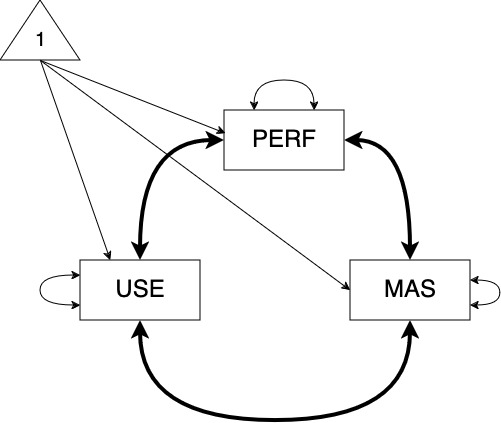
Model 1: Diagram of correlation model with perf, use, and mas
You can check the detailed rules of path analysis diagram here. Some basic rules:
Observed variables: rectangle/square
Latent variables: ellipse/circle
Intercept: triangle shape
Regression relation: single-headed arrow
Correlation/Covariance: double-headed arrow
Point to itself: residual variance
Point to others: covariances
1.2 Homework 2: Model 1 - Correlation Model with perf, use, and mas
model04.syntax ="# Variances:perf ~~ perf use ~~ use mas ~~ mas# Covariance:perf ~~ useperf ~~ masuse ~~ mas# Means:perf ~ 1 use ~ 1 mas ~ 1 "## Estimation for model01model04.fit <-cfa(model04.syntax, data=dataMath, mimic="MPLUS", fixed.x =TRUE, estimator ="MLR") ## Print outputstandardizedsolution(model04.fit)
   lhs op  rhs est.std    se      z pvalue ci.lower ci.upper
1 perf ~~ perf   1.000 0.000     NA     NA    1.000    1.000
2  use ~~  use   1.000 0.000     NA     NA    1.000    1.000
3  mas ~~  mas   1.000 0.000     NA     NA    1.000    1.000
4 perf ~~  use   0.158 0.059  2.685  0.007    0.043    0.273
5 perf ~~  mas   0.526 0.043 12.372  0.000    0.443    0.610
6  use ~~  mas   0.299 0.049  6.109  0.000    0.203    0.395
7 perf ~1        4.719 0.204 23.106  0.000    4.319    5.119
8  use ~1        3.330 0.143 23.257  0.000    3.050    3.611
9  mas ~1        2.797 0.126 22.151  0.000    2.550    3.044
## filter correlations among varaiblesstandardizedsolution(model04.fit) |>filter(op =="~~", lhs != rhs)
   lhs op rhs est.std    se      z pvalue ci.lower ci.upper
1 perf ~~ use   0.158 0.059  2.685  0.007    0.043    0.273
2 perf ~~ mas   0.526 0.043 12.372  0.000    0.443    0.610
3  use ~~ mas   0.299 0.049  6.109  0.000    0.203    0.395
For Performance and Usefulness, there is a weak but significantly positive correlation with r = .158 (.059), p = .007
For Performance and Anxiety, there is a strong and significantly positive correlation with r = .526 (.043), p < .001
For Usefulness and Anxiety, there is a moderate and significantly positive correlation with r = .299 (.049), p < .001
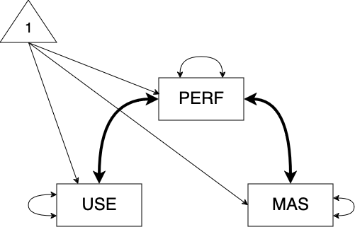
1.3 Homework 2: Model 2 - constraining the correlation of use and mas to 0
Model 2: Constrained model
model04b.syntax ="# Variances:perf ~~ perf use ~~ use mas ~~ mas# Covariance:perf ~~ useperf ~~ masuse ~~ 0*mas# Means:perf ~ 1 use ~ 1 mas ~ 1 "model04b.fit <-cfa(model04b.syntax, data=dataMath, mimic="MPLUS", fixed.x =TRUE, estimator ="MLR") ## Print outputstandardizedsolution(model04b.fit)
   lhs op  rhs est.std    se      z pvalue ci.lower ci.upper
1 perf ~~ perf   1.000 0.000     NA     NA    1.000    1.000
2  use ~~  use   1.000 0.000     NA     NA    1.000    1.000
3  mas ~~  mas   1.000 0.000     NA     NA    1.000    1.000
4 perf ~~  use   0.017 0.056  0.298  0.765   -0.092    0.126
5 perf ~~  mas   0.523 0.044 11.790  0.000    0.436    0.610
6  use ~~  mas   0.000 0.000     NA     NA    0.000    0.000
7 perf ~1        4.730 0.206 22.993  0.000    4.327    5.134
8  use ~1        3.325 0.143 23.212  0.000    3.044    3.606
9  mas ~1        2.790 0.127 22.056  0.000    2.542    3.038
   lhs op rhs est.std    se      z pvalue ci.lower ci.upper
1 perf ~~ use   0.017 0.056  0.298  0.765   -0.092    0.126
2 perf ~~ mas   0.523 0.044 11.790  0.000    0.436    0.610
3  use ~~ mas   0.000 0.000     NA     NA    0.000    0.000
For Performance and Usefulness, there is a weak and non-significantly positive correlation with r = .017 (.056), p = .765
For Performance and Anxiety, there is a strong and significantly positive correlation with r = .523 (.044), p < .001
For Usefulness and Anxiety, there is a zero correlation with r = 0 (0), p = NA
1.4 Homework 2: AIC and BIC
anova(model04.fit, model04b.fit)
Scaled Chi-Squared Difference Test (method = "satorra.bentler.2001")

lavaan NOTE:
    The "Chisq" column contains standard test statistics, not the
    robust test that should be reported per model. A robust difference
    test is a function of two standard (not robust) statistics.

             Df    AIC    BIC  Chisq Chisq diff Df diff Pr(>Chisq)
model04.fit   0 6421.3 6456.0  0.000
model04b.fit  1 6446.5 6477.4 27.234     29.031       1  7.123e-08 ***
---
Signif. codes:  0 '***' 0.001 '**' 0.01 '*' 0.05 '.' 0.1 ' ' 1
For Model 1, AIC = 6421.3 and BIC = 6456.0
For Model 2, AIC = 6446.5 and BIC = 6477.4
According to the criteria of lower AIC/BIC values indicating better model fit and the result of Likelihood ratio test (\chi^2(0, 1)=29.031, p < .001), we prefer model 1 as it has significantly better model fit than model 2.
---title: "Lecture 09: Path Analysis"subtitle: "Homework 2"author: "Jihong Zhang*, Ph.D"institute: | Educational Statistics and Research Methods (ESRM) Program* University of Arkansasdate: "2024-10-09"date-modified: "2024-10-11"sidebar: falseexecute: echo: true warning: falseoutput-location: defaultcode-annotations: belowhighlight-style: "nord"format: html: page-layout: full toc: true toc-depth: 2 toc-expand: true lightbox: true code-fold: false fig-align: center---# Homework 2```{r}#| output-location: defaultlibrary(ESRM64503)library(kableExtra)library(tidyverse)library(DescTools) # Desc() allows you to quick screen datalibrary(lavaan) # Desc() allows you to quick screen data# options(digits = 3)head(dataMath)dim(dataMath)```## Homework 2: Setup{fig-align="center"}You can check the detailed rules of path analysis diagram [here](https://websem.psychstat.org/wiki/_media/manual/websem-draw-pathdiagrams.pdf). Some basic rules:1. Observed variables: rectangle/square2. Latent variables: ellipse/circle3. Intercept: triangle shape4. Regression relation: single-headed arrow5. Correlation/Covariance: double-headed arrow 1. Point to itself: residual variance 2. Point to others: covariances## Homework 2: Model 1 - Correlation Model with perf, use, and mas```{r}#| output-location: columnmodel04.syntax ="# Variances:perf ~~ perf use ~~ use mas ~~ mas# Covariance:perf ~~ useperf ~~ masuse ~~ mas# Means:perf ~ 1 use ~ 1 mas ~ 1 "## Estimation for model01model04.fit <-cfa(model04.syntax, data=dataMath, mimic="MPLUS", fixed.x =TRUE, estimator ="MLR") ## Print outputstandardizedsolution(model04.fit)## filter correlations among varaiblesstandardizedsolution(model04.fit) |>filter(op =="~~", lhs != rhs)```- For Performance and Usefulness, there is a weak but significantly positive correlation with **r = .158 (.059), p = .007**- For Performance and Anxiety, there is a strong and significantly positive correlation with **r = .526 (.043), p \< .001**- For Usefulness and Anxiety, there is a moderate and significantly positive correlation with **r = .299 (.049), p \< .001**## Homework 2: Model 2 - constraining the correlation of use and mas to 0{fig-align="center"}```{r}model04b.syntax ="# Variances:perf ~~ perf use ~~ use mas ~~ mas# Covariance:perf ~~ useperf ~~ masuse ~~ 0*mas# Means:perf ~ 1 use ~ 1 mas ~ 1 "model04b.fit <-cfa(model04b.syntax, data=dataMath, mimic="MPLUS", fixed.x =TRUE, estimator ="MLR") ## Print outputstandardizedsolution(model04b.fit)standardizedsolution(model04b.fit) |>filter(op =="~~", lhs != rhs)```- For Performance and Usefulness, there is a weak and non-significantly positive correlation with **r = .017 (.056), p = .765**- For Performance and Anxiety, there is a strong and significantly positive correlation with **r = .523 (.044), p \< .001**- For Usefulness and Anxiety, there is a zero correlation with **r = 0 (0), p = NA**## Homework 2: AIC and BIC```{r}anova(model04.fit, model04b.fit)```- For Model 1, AIC = 6421.3 and BIC = 6456.0- For Model 2, AIC = 6446.5 and BIC = 6477.4- According to the criteria of lower AIC/BIC values indicating better model fit and the result of Likelihood ratio test ($\chi^2(0, 1)=29.031, p < .001$), we prefer model 1 as it has significantly better model fit than model 2.