[1] 0.6Lecture 11: Introduction to Bayesian Statistics and Markov Chain Monte Carlo Estimation
Educational Statistics and Research Methods (ESRM) Program*
University of Arkansas
2024-10-09
Today’s Lecture Objectives
Bayes’ Theorem
Likelihood function vs. Posterior distribution
How to report posterior distribution of parameters
Bayesian update
Bayesian Linear Regression and Multivariate Regression
Brief Introduction to Bayesian
What is Bayesian?
- A statistical inference based on Bayesian Probability Theory to estimate uncertainty
What are key components of Bayesian models?
- Likelihood function - likelihood of data given assumed probability distribution
- Prior distribution - belief / previous evidences of parameters
- Posterior distribution - updated information of parameters given our data and modeling
- Posterior predictive distribution - future / predicted data
What are the differences between Bayesian with Frequentist analysis?
- Input: prior distribution: Bayesian vs. hypothesis of fixed parameters: frequentist
- Estimation process: Markov Chain Monte Carlo (MCMC) vs. Maximum Likelihood Estimation (MLE)
- Result: posterior distribution vs. point estimates of parameters
- Accuracy check: credible interval (plausibility of the parameters having those values) vs. confidence interval (the proportion of infinite samples having the fixed parameters)
Bayes’ Theorem: How Bayesian Statistics Work
Bayesian methods rely on Bayes’ Theorem
\[ P(\boldsymbol{\theta} | Data) = \frac{P(Data|\boldsymbol{\theta})P(\boldsymbol{\theta})}{P(Data)} \propto P(Data|\boldsymbol{\theta}) P(\boldsymbol{\theta}) \]
Where:
- P: probability distribution function (PDF)
- \(P(\boldsymbol{\theta}|Data)\) : the posterior distribution of parameter \(\boldsymbol{\theta}\), given the observed data
- \(P(Data|\boldsymbol{\theta})\): the likelihood function (conditional distributin) of the observed data, given the parameters
- \(P(\boldsymbol{\theta})\): the prior distribution of parameter \(\boldsymbol{\theta}\)
- \(P(Data)\): the marginal distribution of the observed data
A Live Bayesian Example
Suppose we want to assess the probability of rolling a “1” on a six-sided die:
\[ \boldsymbol{\theta} \equiv p_{1} = P(D = 1) \]
Suppose we collect a sample of data (N = 5):
\[Data \equiv X = \{0, 1, 0, 1, 1\}\]The prior distribution of parameters is denoted as \(P(p_1)\): how much the probability of “1” will occur we “believe” ;
The likelihood function is denoted as \(P(X | p_1)\);
The posterior distribution is denoted as \(P(p_1|X)\)
The aim of Bayesian is to estimate the probability of rolling a “1” give the Data (posterior distribution) as:
\[ P(p_1|X) = \frac{P(X|p_1)P(p_1)}{P(X)} \propto P(X|p_1) P(p_1) \]
Why use Bayesian
- Bayesian approach to statistics is more intuitive; it resembles how we think about probability in everyday life (our prior belif and our updated belief after observing the data) – in the odds of hypotheses, not those of data. In comparison, the frequentist conclusion sounds complex and difficult to comprehend.
- Bayesian approach is much easier to construct very complicated model: using MCMC, we did not need to derive likelihood function by ourselves.
- Bayesian approach is very flexible to incorporate prior (old, history) data; while the frequentist inference is static, which only use current data.
Step 1: Choose the Likelihood function (Model)
The Likelihood function \(P(X|p_1)\) follows Binomial distribution of 3 successes out of 5 samples:
\[P(X|p_1) = \prod_{i =1}^{N=5} p_1^{X_i}(1-p_1)^{X_i} \\= (1-p_i) \cdot p_i \cdot (1-p_i) \cdot p_i \cdot p_i\]We use Bernoulli (Binomial) Distribution (feat. Jacob Bernoulli, 1654-1705) because Bernoulli dist. has nice statistical probability.
- “Nice” means making totally sense in normal life– a common belief. For example, the \(p_1\) value that maximizes the Bernoulli-based likelihood function is \(Mean(X)\), and the \(p_1\) values that minimizes the Bernoulli-based likelihood function is 0 or 1
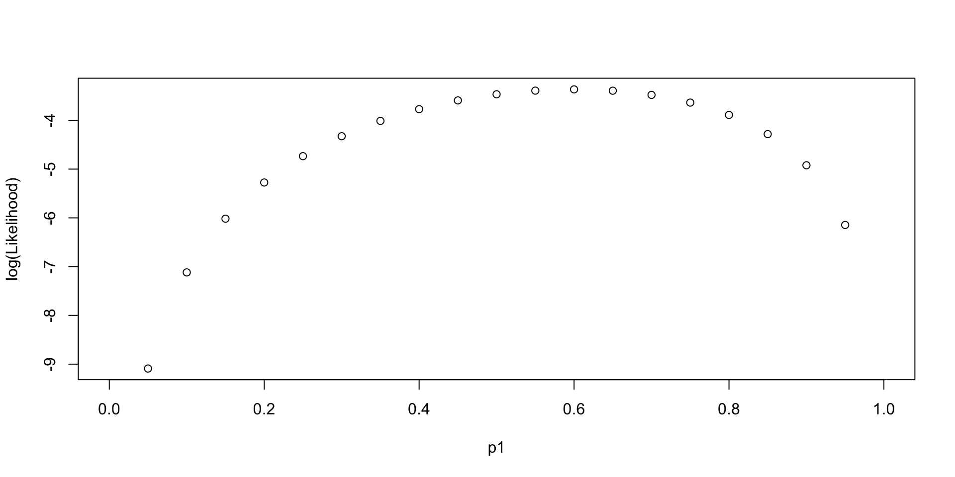
Log-likelihood Function across different values of Parameter
\[ LL(p_1, Data =\{0, 1, 0, 1, 1\}) \]
Log-likelihood Function given different Data sets
\[ LL(p_1 \in \{0, 0.2,0.4, 0.6, 0.8,1\}, Data \in \{0/5, 1/5, 2/5, 3/5, 4/5, 5/5\}) \]
Code
library(tidyverse)
p1 = c(0, 2, 4, 6, 8, 10) / 10
nTrails = 5
nSuccess = 0:nTrails
Likelihood = sapply(p1, \(x) choose(nTrails,nSuccess)*(x)^nSuccess*(1-x)^(nTrails - nSuccess))
Likelihood_forPlot <- as.data.frame(Likelihood)
colnames(Likelihood_forPlot) <- p1
Likelihood_forPlot$Sample = factor(paste0(nSuccess, " out of ", nTrails), levels = paste0(nSuccess, " out of ", nTrails))
# plot
Likelihood_forPlot %>%
  pivot_longer(-Sample, names_to = "p1") %>%
  mutate(`log(Likelihood)` = log(value)) %>%
  ggplot(aes(x = Sample, y = `log(Likelihood)`, color = p1)) +
  geom_point(size = 2) +
  geom_path(aes(group=p1), size = 1.3)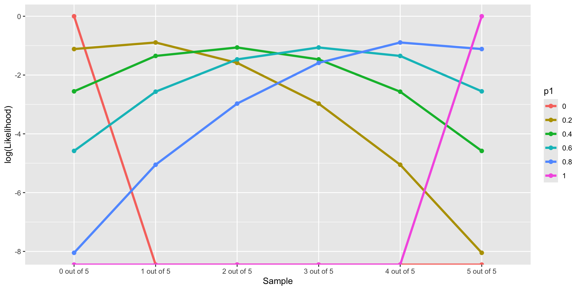
Step 2: Choose the Prior Distribution for \(p_1\)
We must now pick the prior distribution of \(p_1\):
\[ P(p_1) \]
Compared to likelihood function, we have much more choices. Many distributions to choose from
To choose prior distribution, think about what we know about a “fair” die.
the probability of rolling a “1” is about \(\frac{1}{6}\)
the probabilities much higher/lower than \(\frac{1}{6}\) are very unlikely
Let’s consider a Beta distribution:
\[ p_1 \sim Beta(\alpha, \beta) \]
Prior for probability parameter: The Beta Distribution
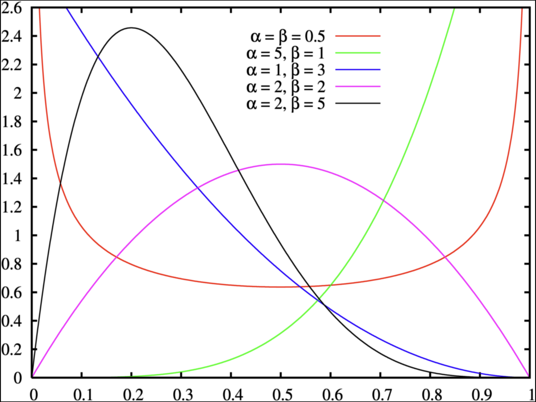
For parameters that range between 0 and 1, the beta distribution with two hyperparameters {\(\alpha\), \(\beta\)} makes a good choice for prior distribution:
\[ P(p_1) = \frac{(p_1)^{a-1} (1-p_1)^{\beta-1}}{B(\alpha,\beta)} \]
Where denominator \(B\) is:
\[ B(\alpha,\beta) = \frac{\Gamma(\alpha)\Gamma(\beta)}{\Gamma(\alpha+\beta)} \]
and (fun fact: derived by Daniel Bernoulli (1700-1782)),
\[ \Gamma(\alpha) = \int_0^{\infty}t^{\alpha-1}e^{-t}dt \]
More nice properties: Beta Distribution
The Beta distribution has a mean of \(\frac{\alpha}{\alpha+\beta}\) and a mode of \(\frac{\alpha -1}{\alpha + \beta -2}\) for \(\alpha > 1\) & \(\beta > 1\); (fun fact: when \(\alpha\ \&\ \beta< 1\), pdf is U-shape, what that mean?)
\(\alpha\) and \(\beta\) are called hyperparameters of the parameter \(p_1\);
Hyperparameters are parameters of prior parameters ;
When \(\alpha = \beta = 1\), the distribution is uniform distribution;
To make sure \(P(p_1 = \frac{1}{6})\) is the largest, we can:
Many choices: \(\alpha =2\) and \(\beta = 6\) has the same mode as \(\alpha = 100\) and \(\beta = 496\); (hint: \(\beta = 5\alpha - 4\))
The differences between choices is how strongly we feel in our beliefs
Conjugacy of Beta Distribution
When the binomial likelihood is multiplied by the beta prior, the result is proportional to another beta distribution:
- \(\text{Posterior} \propto \theta^x (1 - \theta)^{n-x} \times \theta^{\alpha - 1} (1 - \theta)^{\beta - 1}\)
- Simplifies to: \(\theta^{x + \alpha - 1} (1 - \theta)^{n - x + \beta - 1}\)
This is the kernel of a beta distribution with updated parameters \(\alpha' = x + \alpha\) and \(\beta' = n - x + \beta\). The fact that the posterior is still a beta distribution is what makes the beta distribution a conjugate prior for the binomial likelihood.
Human langauge: Both beta (prior) and binomial (likelihood) are so-called “exponetial family”. The muliplication of them is still a “exponential family” distribution.
How strongly we believe in the prior
- The Beta distribution has a variance of \(\frac{\alpha\beta}{(\alpha+\beta)^2 (\alpha + \beta + 1)}\)
- The smaller prior variance means the prior is more informative
- Informative priors are those that have relatively small variances
- Uninformative priors are those that have relatively large variances
- Suppose we have four sets of hyperparameters choices: (2,6);(20,96);(100,496);(200,996)
Code
# Function for variance of Beta distribution
varianceFun = function(alpha_beta){
  alpha = alpha_beta[1]
  beta = alpha_beta[2]
  return((alpha * beta)/((alpha + beta)^2*(alpha + beta + 1)))
}

# Multiple prior choices from uninformative to informative
alpha_beta_choices = list(
  I_dont_trust = c(2, 6),
  not_strong =   c(20, 96),
  litte_strong = c(100, 496),
  very_strong =  c(200, 996))

## Transform to data.frame for plot
alpha_beta_variance_plot <- t(sapply(alpha_beta_choices, varianceFun)) %>%
  as.data.frame() %>%
  pivot_longer(everything(), names_to = "Degree", values_to = "Variance") %>%
  mutate(Degree = factor(Degree, levels = unique(Degree))) %>%
  mutate(Alpha_Beta = c(
    "(2, 6)",
    "(20, 96)",
    "(100, 496)",
    "(200, 996)"
  ))

alpha_beta_variance_plot %>%
  ggplot(aes(x = Degree, y = Variance)) +
  geom_col(aes(fill = Degree)) +
  geom_text(aes(label = Alpha_Beta), size = 6) +
  labs(title = "Variances along difference choices of alpha and beta") +
theme(text = element_text(size = 21)) 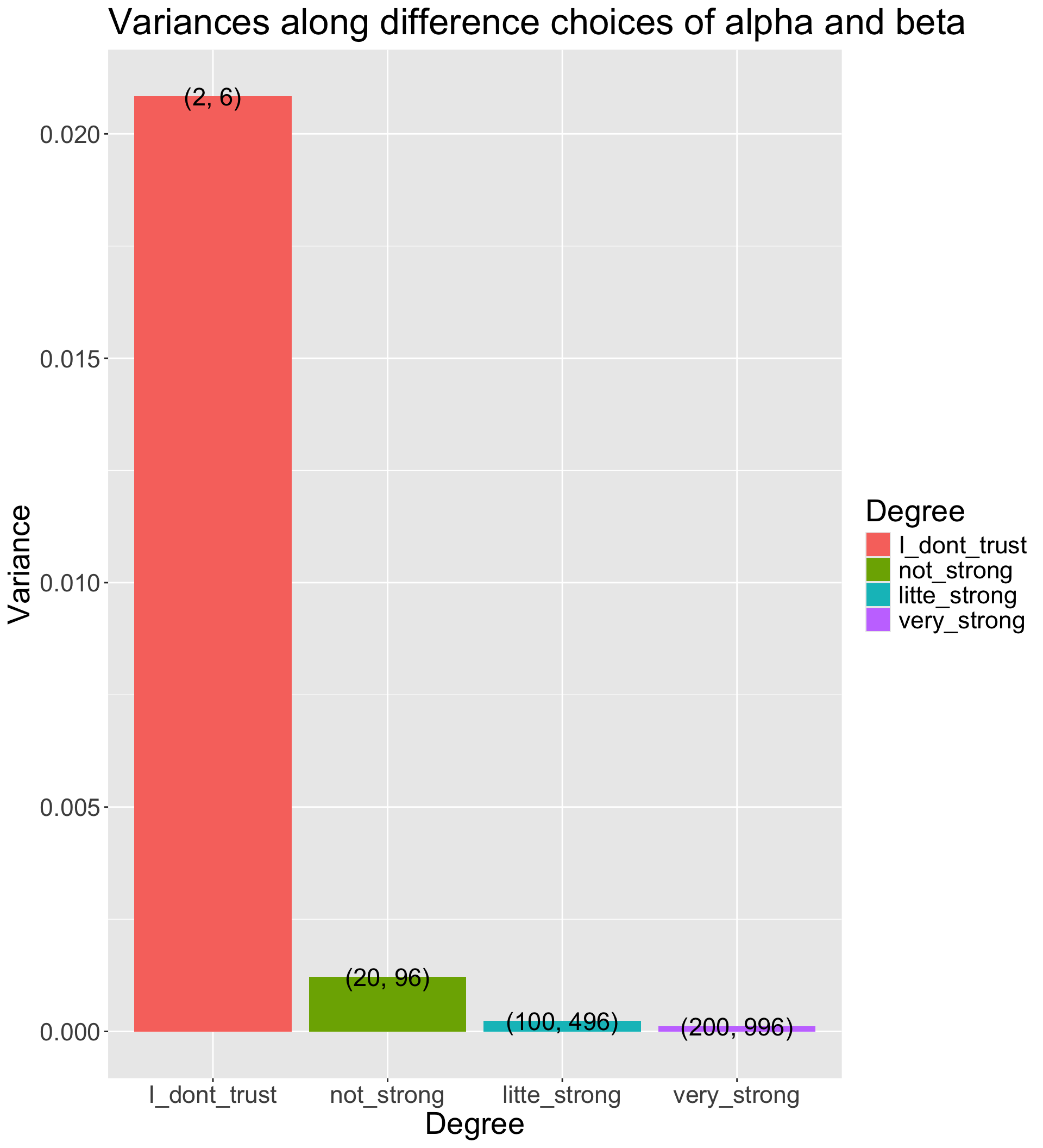
Visualize prior distribution \(P(p_1)\)
Code
dbeta <- function(p1, alpha, beta) {
  # probability density function
  PDF = ((p1)^(alpha-1)*(1-p1)^(beta-1)) / beta(alpha, beta)
  return(PDF)
}

condition <- data.frame(
  alpha = c(2, 20, 100, 200),
  beta = c(6, 96, 496, 996)
)
pdf_bycond <- condition %>%
  nest_by(alpha, beta) %>%
  mutate(data = list(
    dbeta(p1 = (1:99)/100, alpha = alpha, beta = beta)
  ))

## prepare data for plotting pdf by conditions
pdf_forplot <- Reduce(cbind, pdf_bycond$data) %>%
  t() %>%
  as.data.frame() ## merge conditions together
colnames(pdf_forplot) <- (1:99)/100 # add p1 values as x-axis
pdf_forplot <- pdf_forplot %>%
  mutate(Alpha_Beta = c( # add alpha_beta conditions as colors
    "(2, 6)",
    "(20, 96)",
    "(100, 496)",
    "(200, 996)"
  )) %>%
  pivot_longer(-Alpha_Beta, names_to = 'p1', values_to = 'pdf') %>%
  mutate(p1 = as.numeric(p1),
         Alpha_Beta = factor(Alpha_Beta,levels = unique(Alpha_Beta)))

pdf_forplot %>%
  ggplot() +
  geom_vline(xintercept = 0.17, col = "black") +
  geom_point(aes(x = p1, y = pdf, col = Alpha_Beta)) +
  geom_path(aes(x = p1, y = pdf, col = Alpha_Beta, group = Alpha_Beta)) +
  scale_color_discrete(name = "Prior choices")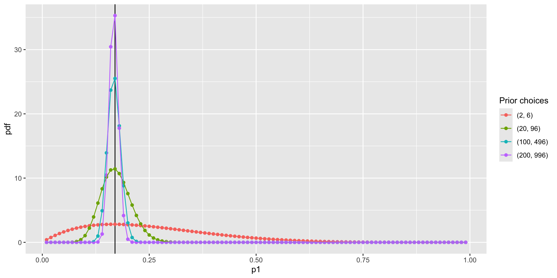
Question: WHY NOT USE NORMAL DISTRIBUTION?
Step 3: The Posterior Distribution
Choose a Beta distribution as the prior distribution of \(p_1\) is very convenient:
When combined with Bernoulli (Binomial) data likelihood, the posterior distribution (\(P(p_1|Data)\)) can be derived analytically
The posterior distribution is also a Beta distribution
\(\alpha' = \alpha + \sum_{i=1}^{N}X_i\) (\(\alpha'\) is parameter of the posterior distribution)
\(\beta' = \beta + (N - \sum_{i=1}^{N}X_i)\) (\(\beta'\) is parameter of the posterior distribution)
The Beta distribution is said to be a conjugate prior in Bayesian analysis: A prior distribution that leads to posterior distribution of the same family
- Prior and Posterior distribution are all Beta distribution
Visualize the posterior distribution \(P(p_1|Data)\)
Code
dbeta_posterior <- function(p1, alpha, beta, data) {
  alpha_new = alpha + sum(data)
  beta_new = beta + (length(data) - sum(data) )
  # probability density function
  PDF = ((p1)^(alpha_new-1)*(1-p1)^(beta_new-1)) / beta(alpha_new, beta_new)
  return(PDF)
}
# Observed data
dat = c(0, 1, 0, 1, 1)

condition <- data.frame(
  alpha = c(2, 20, 100, 200),
  beta = c(6, 96, 496, 996)
)

pdf_posterior_bycond <- condition %>%
  nest_by(alpha, beta) %>%
  mutate(data = list(
    dbeta_posterior(p1 = (1:99)/100, alpha = alpha, beta = beta,
                    data = dat)
  ))

## prepare data for plotting pdf by conditions
pdf_posterior_forplot <- Reduce(cbind, pdf_posterior_bycond$data) %>%
  t() %>%
  as.data.frame() ## merge conditions together
colnames(pdf_posterior_forplot) <- (1:99)/100 # add p1 values as x-axis
pdf_posterior_forplot <- pdf_posterior_forplot %>%
  mutate(Alpha_Beta = c( # add alpha_beta conditions as colors
    "(2, 6)",
    "(20, 96)",
    "(100, 496)",
    "(200, 996)"
  )) %>%
  pivot_longer(-Alpha_Beta, names_to = 'p1', values_to = 'pdf') %>%
  mutate(p1 = as.numeric(p1),
         Alpha_Beta = factor(Alpha_Beta,levels = unique(Alpha_Beta)))

pdf_posterior_forplot %>%
  ggplot() +
  geom_vline(xintercept = 0.17, col = "black") +
  geom_point(aes(x = p1, y = pdf, col = Alpha_Beta)) +
  geom_path(aes(x = p1, y = pdf, col = Alpha_Beta, group = Alpha_Beta)) +
  scale_color_discrete(name = "Prior choices") +
  labs( y = '')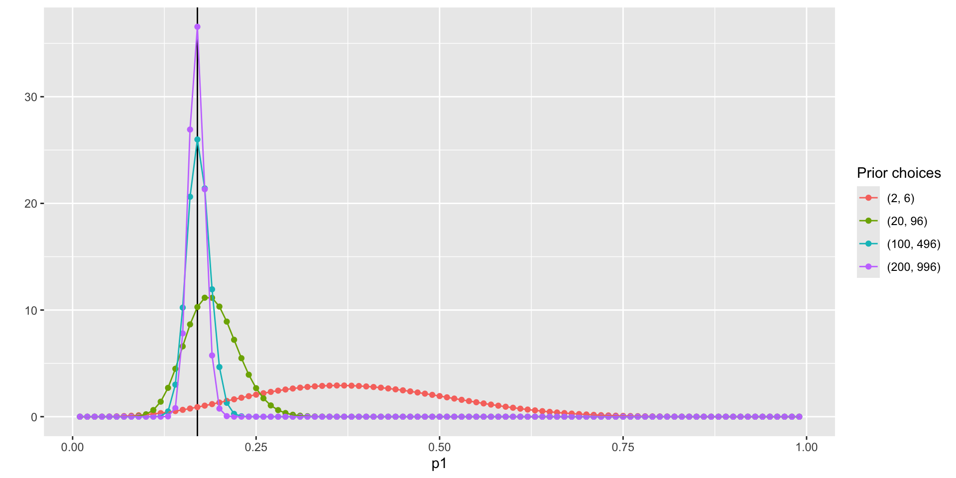
Manually calculate summaries of the posterior distribution
To determine the estimate of \(p_1\) using data \(\{0, 1, 0, 1,1\}\), we need to summarize the posterior distribution:
With prior hyperparameters \(\alpha = 2\) and \(\beta = 6\) and the data \(\sum_{i=1}^{N}X = 3\) and \(N = 5\):
\(\hat p_1 = \frac{\alpha'}{\alpha' + \beta'}= \frac{2+3}{2+3+6+2}=\frac{5}{13} = .3846\)
SD = 0.1300237
With prior hyperparameters \(\alpha = 100\) and \(\beta = 496\):
\(\hat p_1 = \frac{100+3}{100+3+496+2}=\frac{103}{601} = .1714\)
SD = 0.0153589
Bayesian Analysis in R: Stan Program
Introduction to Stan
Stan is a widely used MCMC estimation program
Most recent; has many convenient features
Actually does several methods of estimation (ML, Variational Bayes)
You create a model using Stan’s syntax
Stan translates your model to a custom-built C++ syntax
Stan then compiles your model into its own executable program
You then run the program to estimate your model
- If you use R, the interface can be seamless
Stan and Rstudio
Option 1: Stan has its own syntax which can be built in stand-alone text files (.stan)
Rstudio will let you create a stan file in the new
FilemenuRstudio also has syntax highlighting in Stan files
Save
.stanto the same path of your.r
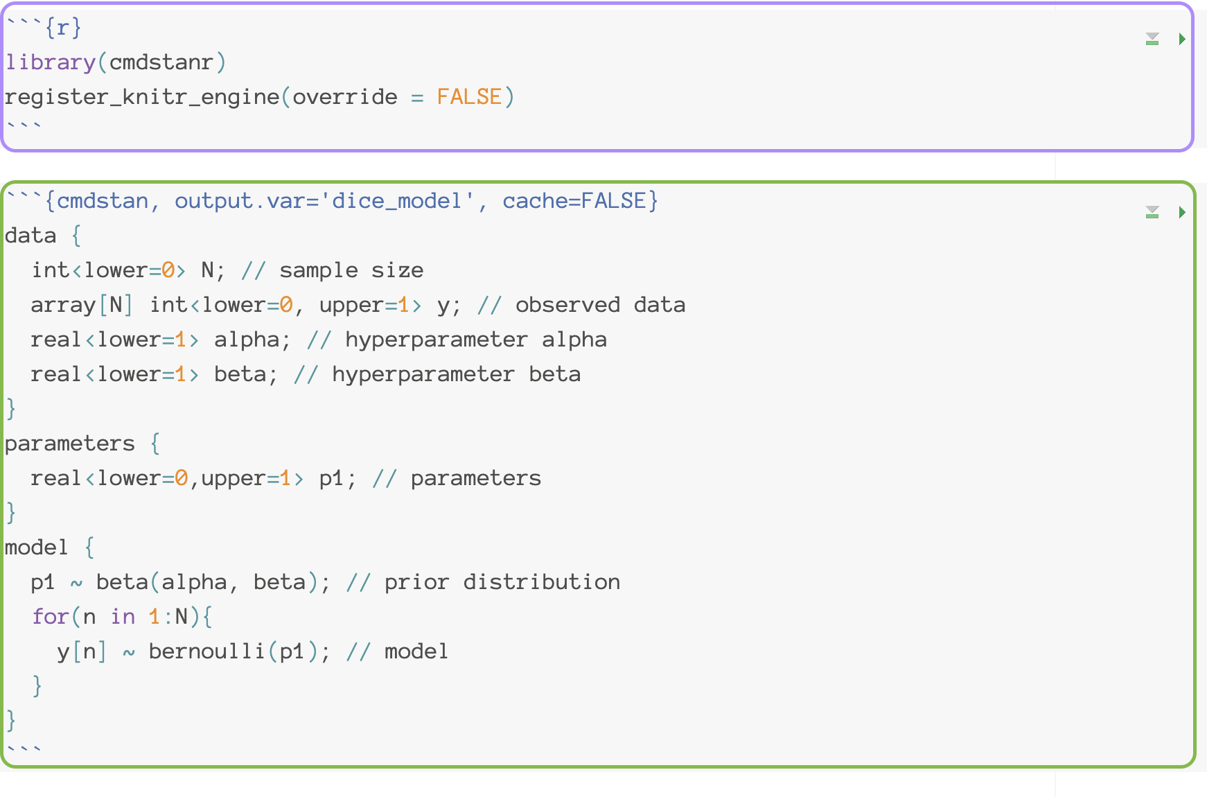
Option 2: You can also use Stan in a interactive way in qmd file
- Which is helpful when you want to test multiple stan models and report your results at the same time

Install CmdStan
Stan Code for the example model
data {
  int<lower=0> N; // sample size
  array[N] int<lower=0, upper=1> y; // observed data
  real<lower=1> alpha; // hyperparameter alpha
  real<lower=1> beta; // hyperparameter beta
}
parameters {
  real<lower=0,upper=1> p1; // parameters
}
model {
  p1 ~ beta(alpha, beta); // prior distribution
  for(n in 1:N){
    y[n] ~ bernoulli(p1); // model
  }
}
# mod <- cmdstan_model('dice_model.stan')
data_list1 <- list(
y = c(0, 1, 0, 1, 1),
N = 5,
alpha = 2,
beta = 6
)
data_list2 <- list(
y = c(0, 1, 0, 1, 1),
N = 5,
alpha = 100,
beta = 496
)
fit1 <- dice_model$sample(
data = data_list1,
seed = 123,
chains = 4,
parallel_chains = 4,
refresh = 1000
)Running MCMC with 4 parallel chains...
Chain 1 Iteration: 1 / 2000 [ 0%] (Warmup)
Chain 1 Iteration: 1000 / 2000 [ 50%] (Warmup)
Chain 1 Iteration: 1001 / 2000 [ 50%] (Sampling)
Chain 1 Iteration: 2000 / 2000 [100%] (Sampling)
Chain 2 Iteration: 1 / 2000 [ 0%] (Warmup)
Chain 2 Iteration: 1000 / 2000 [ 50%] (Warmup)
Chain 2 Iteration: 1001 / 2000 [ 50%] (Sampling)
Chain 2 Iteration: 2000 / 2000 [100%] (Sampling)
Chain 3 Iteration: 1 / 2000 [ 0%] (Warmup)
Chain 3 Iteration: 1000 / 2000 [ 50%] (Warmup)
Chain 3 Iteration: 1001 / 2000 [ 50%] (Sampling)
Chain 3 Iteration: 2000 / 2000 [100%] (Sampling)
Chain 4 Iteration: 1 / 2000 [ 0%] (Warmup)
Chain 4 Iteration: 1000 / 2000 [ 50%] (Warmup)
Chain 4 Iteration: 1001 / 2000 [ 50%] (Sampling)
Chain 4 Iteration: 2000 / 2000 [100%] (Sampling)
Chain 1 finished in 0.0 seconds.
Chain 2 finished in 0.0 seconds.
Chain 3 finished in 0.0 seconds.
Chain 4 finished in 0.0 seconds.
All 4 chains finished successfully.
Mean chain execution time: 0.0 seconds.
Total execution time: 0.2 seconds.fit2 <- dice_model$sample(
data = data_list2,
seed = 123,
chains = 4,
parallel_chains = 4,
refresh = 1000
)Running MCMC with 4 parallel chains...
Chain 1 Iteration: 1 / 2000 [ 0%] (Warmup)
Chain 1 Iteration: 1000 / 2000 [ 50%] (Warmup)
Chain 1 Iteration: 1001 / 2000 [ 50%] (Sampling)
Chain 1 Iteration: 2000 / 2000 [100%] (Sampling)
Chain 2 Iteration: 1 / 2000 [ 0%] (Warmup)
Chain 2 Iteration: 1000 / 2000 [ 50%] (Warmup)
Chain 2 Iteration: 1001 / 2000 [ 50%] (Sampling)
Chain 2 Iteration: 2000 / 2000 [100%] (Sampling)
Chain 3 Iteration: 1 / 2000 [ 0%] (Warmup)
Chain 3 Iteration: 1000 / 2000 [ 50%] (Warmup)
Chain 3 Iteration: 1001 / 2000 [ 50%] (Sampling)
Chain 3 Iteration: 2000 / 2000 [100%] (Sampling)
Chain 4 Iteration: 1 / 2000 [ 0%] (Warmup)
Chain 4 Iteration: 1000 / 2000 [ 50%] (Warmup)
Chain 4 Iteration: 1001 / 2000 [ 50%] (Sampling)
Chain 4 Iteration: 2000 / 2000 [100%] (Sampling)
Chain 1 finished in 0.0 seconds.
Chain 2 finished in 0.0 seconds.
Chain 3 finished in 0.0 seconds.
Chain 4 finished in 0.0 seconds.
All 4 chains finished successfully.
Mean chain execution time: 0.0 seconds.
Total execution time: 0.2 seconds.Uninformative prior distribution (2, 6) and posterior distribution
Code
bayesplot::mcmc_dens(fit1$draws('p1')) +
  geom_path(aes(x = p1, y = pdf), data = pdf_posterior_forplot %>% filter(Alpha_Beta == '(2, 6)'), col = "red") +
  geom_vline(xintercept = 1/6, col = "green") +
  geom_vline(xintercept = 3/5, col = "purple") +
labs(title = "Posterior distribution using uninformative prior vs. the conjugate prior (The Gibbs sampler) method", caption = 'Green: mode of prior distribution; Purple: expected value from observed data; Red: Gibbs sampling method')# A tibble: 2 × 10
variable mean median sd mad q5 q95 rhat ess_bulk ess_tail
<chr> <dbl> <dbl> <dbl> <dbl> <dbl> <dbl> <dbl> <dbl> <dbl>
1 lp__ -9.19 -8.91 0.751 0.337 -10.7 -8.66 1.00 1812. 2400.
2 p1 0.383 0.377 0.131 0.137 0.180 0.609 1.00 1593. 1629.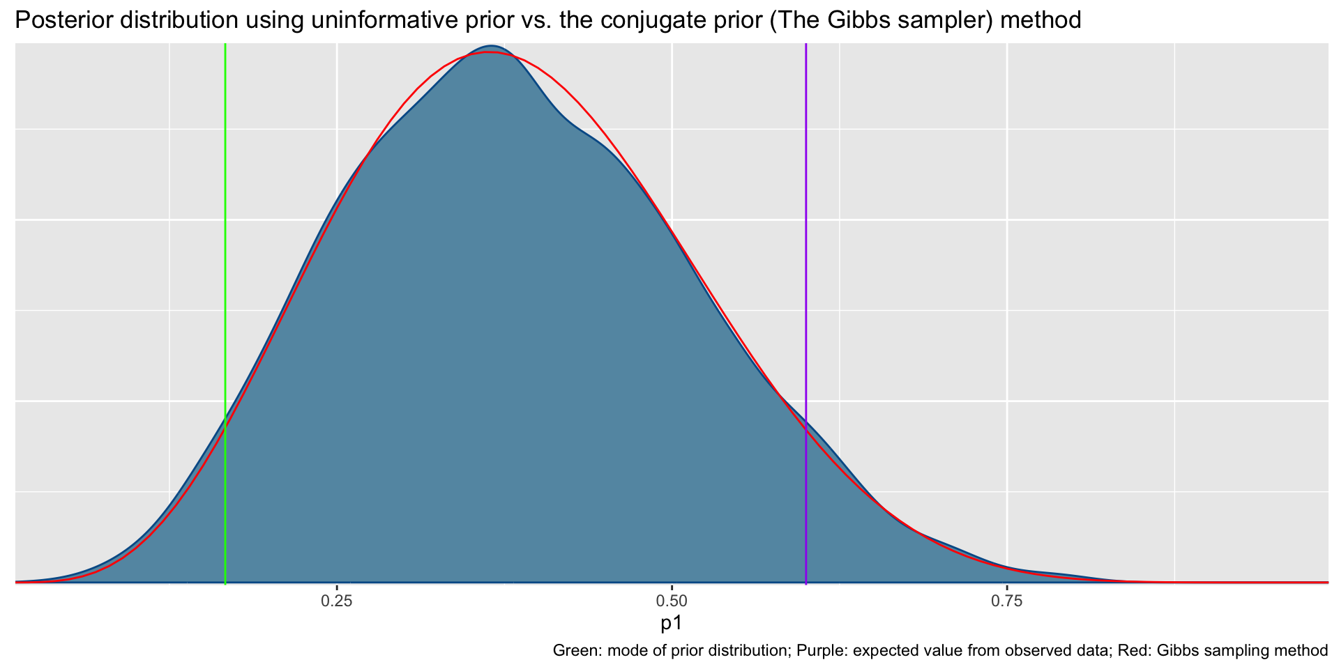
Informative prior distribution (100, 496) and posterior distribution
Code
bayesplot::mcmc_dens(fit2$draws('p1')) +
  geom_path(aes(x = p1, y = pdf), data = pdf_posterior_forplot %>% filter(Alpha_Beta == '(100, 496)'), col = "red") +
  geom_vline(xintercept = 1/6, col = "green") +
  geom_vline(xintercept = 3/5, col = "purple") +
labs(title = "Posterior distribution using informative prior vs. the conjugate prior (The Gibbs sampler) method", caption = 'Green: mode of prior distribution; Purple: expected value from observed data; Red: Gibbs sampling method')# A tibble: 2 × 10
variable mean median sd mad q5 q95 rhat ess_bulk
<chr> <dbl> <dbl> <dbl> <dbl> <dbl> <dbl> <dbl> <dbl>
1 lp__ -276. -276. 0.716 0.317 -277. -275. 1.00 1816.
2 p1 0.171 0.171 0.0154 0.0155 0.146 0.197 1.00 1627.
# ℹ 1 more variable: ess_tail <dbl>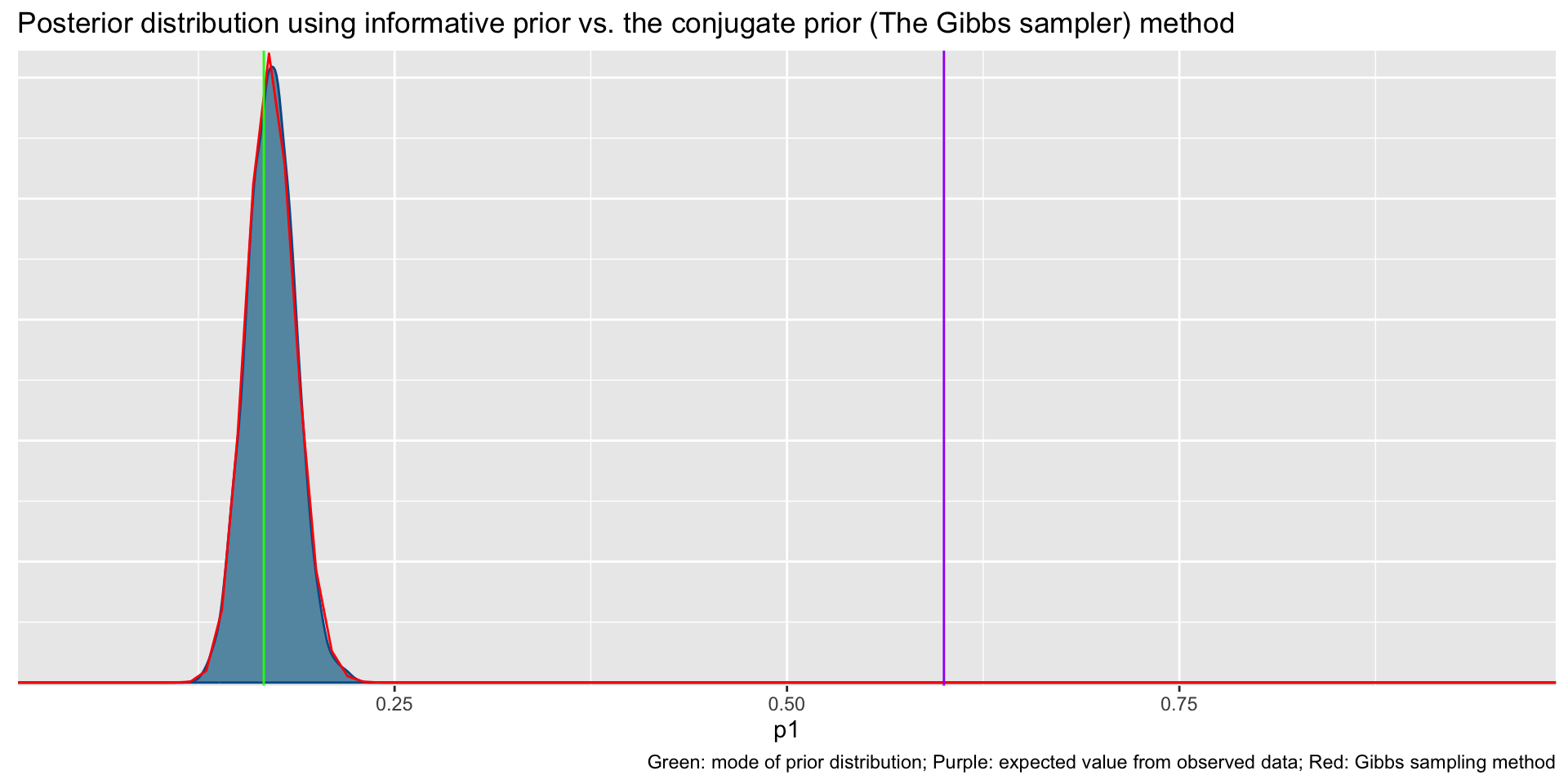
Bayesian updating
We can use the posterior distribution as a prior!
data {0, 1, 0, 1, 1} with the prior hyperparameter {2, 6} -> posterior parameter {5, 9}
new data {1, 1, 1, 1, 1} with the prior hyperparameter {5, 9} -> posterior parameter {10, 9}
one more new data {0, 0, 0, 0, 0} with the prior hyperparameter {10, 9} -> posterior parameter {10, 14}
Bayesian Linear Regression
Our Data Today
library(ESRM64503)
dat <- dataSexHeightWeight
dat$Female <- ifelse(dat$sex == "F", 1, 0)

# Linear Model with Least Squares
## Center independent variable - HeightIN for better interpretation
dat$heightIN <- dat$heightIN - 60

## an empty model suggested by data
EmptyModel <- lm(weightLB ~ 1, data = dat)

## Examine assumptions and leverage of fit
### Residual plot, Q-Q residuals, Scale-Location
# plot(EmptyModel)

## Look at ANOVA table
### F-values, Sum/Mean of square of residuals
# anova(EmptyModel)

## look at parameter summary
summary(EmptyModel)
Call:
lm(formula = weightLB ~ 1, data = dat)

Residuals:
   Min     1Q Median     3Q    Max
 -74.4  -52.4   -8.4   53.1   85.6

Coefficients:
            Estimate Std. Error t value Pr(>|t|)
(Intercept)   183.40      12.61   14.55 9.43e-12 ***
---
Signif. codes:  0 '***' 0.001 '**' 0.01 '*' 0.05 '.' 0.1 ' ' 1

Residual standard error: 56.38 on 19 degrees of freedom
Stan Syntax for Empty Model
A Stan file saved as EmptyModel.stan
- Each line ends with a semi colon
; - Comments are put in with
// - Each block starts with
block typeand is surrounded by curly brackets{}
stanModel <- "
data {
  int<lower=0> N;
  vector[N] weightLB;
}
parameters {
  real beta0;
  real<lower=0> sigma;
}
model {
  beta0 ~ normal(0, 1000);
  sigma ~ uniform(0, 100000);
  weightLB ~ normal(beta0, sigma);
}
"
1model00.fromString = cmdstan_model(stan_file = write_stan_file(stanModel))- 1
-
the
datablock include the observed information
Prepare data for Empty Model
# build R list containing data for Stan: Must be named what "data" are listed in analysis
stanData = list(
1  N = nrow(dat),
2  weightLB = dat$weightLB
)- 1
-
Sample size,
nrow()calculates the number of rows of data - 2
- Vector of dependent variable
Stan needs the data you declared in you syntax to be able to run
Within R, we can pass this data list to Stan via a list object
The entries in the list should correspond to the data block of the Stan syntax
Run Markov Chains in CmdStanr
# run MCMC chain (sample from posterior)
model00.samples = model00.fromString$sample(
1  data = stanData,
2  seed = 1,
3  chains = 3,
4  parallel_chains = 4,
5  iter_warmup = 2000,
  iter_sampling = 1000
)- 1
- Data list
- 2
- Random number seed
- 3
- Number of chains (and parallel chains)
- 4
- Number of warmup iterations (more details shortly)
- 5
- Number of sampling iterations
Running MCMC with 3 chains, at most 4 in parallel...

Chain 1 Iteration:    1 / 3000 [  0%]  (Warmup)
Chain 1 Iteration:  100 / 3000 [  3%]  (Warmup)
Chain 1 Iteration:  200 / 3000 [  6%]  (Warmup)
Chain 1 Iteration:  300 / 3000 [ 10%]  (Warmup)
Chain 1 Iteration:  400 / 3000 [ 13%]  (Warmup)
Chain 1 Iteration:  500 / 3000 [ 16%]  (Warmup)
Chain 1 Iteration:  600 / 3000 [ 20%]  (Warmup)
Chain 1 Iteration:  700 / 3000 [ 23%]  (Warmup)
Chain 1 Iteration:  800 / 3000 [ 26%]  (Warmup)
Chain 1 Iteration:  900 / 3000 [ 30%]  (Warmup)
Chain 1 Iteration: 1000 / 3000 [ 33%]  (Warmup)
Chain 1 Iteration: 1100 / 3000 [ 36%]  (Warmup)
Chain 1 Iteration: 1200 / 3000 [ 40%]  (Warmup)
Chain 1 Iteration: 1300 / 3000 [ 43%]  (Warmup)
Chain 1 Iteration: 1400 / 3000 [ 46%]  (Warmup)
Chain 1 Iteration: 1500 / 3000 [ 50%]  (Warmup)
Chain 1 Iteration: 1600 / 3000 [ 53%]  (Warmup)
Chain 1 Iteration: 1700 / 3000 [ 56%]  (Warmup)
Chain 1 Iteration: 1800 / 3000 [ 60%]  (Warmup)
Chain 1 Iteration: 1900 / 3000 [ 63%]  (Warmup)
Chain 1 Iteration: 2000 / 3000 [ 66%]  (Warmup)
Chain 1 Iteration: 2001 / 3000 [ 66%]  (Sampling)
Chain 1 Iteration: 2100 / 3000 [ 70%]  (Sampling)
Chain 1 Iteration: 2200 / 3000 [ 73%]  (Sampling)
Chain 1 Iteration: 2300 / 3000 [ 76%]  (Sampling)
Chain 1 Iteration: 2400 / 3000 [ 80%]  (Sampling)
Chain 1 Iteration: 2500 / 3000 [ 83%]  (Sampling)
Chain 1 Iteration: 2600 / 3000 [ 86%]  (Sampling)
Chain 1 Iteration: 2700 / 3000 [ 90%]  (Sampling)
Chain 1 Iteration: 2800 / 3000 [ 93%]  (Sampling)
Chain 1 Iteration: 2900 / 3000 [ 96%]  (Sampling)
Chain 1 Iteration: 3000 / 3000 [100%]  (Sampling)
Chain 2 Iteration:    1 / 3000 [  0%]  (Warmup)
Chain 2 Iteration:  100 / 3000 [  3%]  (Warmup)
Chain 2 Iteration:  200 / 3000 [  6%]  (Warmup)
Chain 2 Iteration:  300 / 3000 [ 10%]  (Warmup)
Chain 2 Iteration:  400 / 3000 [ 13%]  (Warmup)
Chain 2 Iteration:  500 / 3000 [ 16%]  (Warmup)
Chain 2 Iteration:  600 / 3000 [ 20%]  (Warmup)
Chain 2 Iteration:  700 / 3000 [ 23%]  (Warmup)
Chain 2 Iteration:  800 / 3000 [ 26%]  (Warmup)
Chain 2 Iteration:  900 / 3000 [ 30%]  (Warmup)
Chain 2 Iteration: 1000 / 3000 [ 33%]  (Warmup)
Chain 2 Iteration: 1100 / 3000 [ 36%]  (Warmup)
Chain 2 Iteration: 1200 / 3000 [ 40%]  (Warmup)
Chain 2 Iteration: 1300 / 3000 [ 43%]  (Warmup)
Chain 2 Iteration: 1400 / 3000 [ 46%]  (Warmup)
Chain 2 Iteration: 1500 / 3000 [ 50%]  (Warmup)
Chain 2 Iteration: 1600 / 3000 [ 53%]  (Warmup)
Chain 2 Iteration: 1700 / 3000 [ 56%]  (Warmup)
Chain 2 Iteration: 1800 / 3000 [ 60%]  (Warmup)
Chain 2 Iteration: 1900 / 3000 [ 63%]  (Warmup)
Chain 2 Iteration: 2000 / 3000 [ 66%]  (Warmup)
Chain 2 Iteration: 2001 / 3000 [ 66%]  (Sampling)
Chain 2 Iteration: 2100 / 3000 [ 70%]  (Sampling)
Chain 2 Iteration: 2200 / 3000 [ 73%]  (Sampling)
Chain 2 Iteration: 2300 / 3000 [ 76%]  (Sampling)
Chain 2 Iteration: 2400 / 3000 [ 80%]  (Sampling)
Chain 2 Iteration: 2500 / 3000 [ 83%]  (Sampling)
Chain 2 Iteration: 2600 / 3000 [ 86%]  (Sampling)
Chain 2 Iteration: 2700 / 3000 [ 90%]  (Sampling)
Chain 2 Iteration: 2800 / 3000 [ 93%]  (Sampling)
Chain 2 Iteration: 2900 / 3000 [ 96%]  (Sampling)
Chain 2 Iteration: 3000 / 3000 [100%]  (Sampling)
Chain 3 Iteration:    1 / 3000 [  0%]  (Warmup)
Chain 3 Iteration:  100 / 3000 [  3%]  (Warmup)
Chain 3 Iteration:  200 / 3000 [  6%]  (Warmup)
Chain 3 Iteration:  300 / 3000 [ 10%]  (Warmup)
Chain 3 Iteration:  400 / 3000 [ 13%]  (Warmup)
Chain 3 Iteration:  500 / 3000 [ 16%]  (Warmup)
Chain 3 Iteration:  600 / 3000 [ 20%]  (Warmup)
Chain 3 Iteration:  700 / 3000 [ 23%]  (Warmup)
Chain 3 Iteration:  800 / 3000 [ 26%]  (Warmup)
Chain 3 Iteration:  900 / 3000 [ 30%]  (Warmup)
Chain 3 Iteration: 1000 / 3000 [ 33%]  (Warmup)
Chain 3 Iteration: 1100 / 3000 [ 36%]  (Warmup)
Chain 3 Iteration: 1200 / 3000 [ 40%]  (Warmup)
Chain 3 Iteration: 1300 / 3000 [ 43%]  (Warmup)
Chain 3 Iteration: 1400 / 3000 [ 46%]  (Warmup)
Chain 3 Iteration: 1500 / 3000 [ 50%]  (Warmup)
Chain 3 Iteration: 1600 / 3000 [ 53%]  (Warmup)
Chain 3 Iteration: 1700 / 3000 [ 56%]  (Warmup)
Chain 3 Iteration: 1800 / 3000 [ 60%]  (Warmup)
Chain 3 Iteration: 1900 / 3000 [ 63%]  (Warmup)
Chain 3 Iteration: 2000 / 3000 [ 66%]  (Warmup)
Chain 3 Iteration: 2001 / 3000 [ 66%]  (Sampling)
Chain 3 Iteration: 2100 / 3000 [ 70%]  (Sampling)
Chain 3 Iteration: 2200 / 3000 [ 73%]  (Sampling)
Chain 3 Iteration: 2300 / 3000 [ 76%]  (Sampling)
Chain 3 Iteration: 2400 / 3000 [ 80%]  (Sampling)
Chain 3 Iteration: 2500 / 3000 [ 83%]  (Sampling)
Chain 3 Iteration: 2600 / 3000 [ 86%]  (Sampling)
Chain 3 Iteration: 2700 / 3000 [ 90%]  (Sampling)
Chain 3 Iteration: 2800 / 3000 [ 93%]  (Sampling)
Chain 3 Iteration: 2900 / 3000 [ 96%]  (Sampling)
Chain 3 Iteration: 3000 / 3000 [100%]  (Sampling)
Chain 1 finished in 0.0 seconds.
Chain 2 finished in 0.0 seconds.
Chain 3 finished in 0.1 seconds.

All 3 chains finished successfully.
Mean chain execution time: 0.0 seconds.
Total execution time: 0.2 seconds.
Within the compiled program and the data, the next step is to run the Markov Chain Monte Carlo (MCMC) sampling (this is basically equivalent to drawing from a posterior distribution)
In
cmdstanr, running the MCMC sampling comes from the$sample()function that is part of the compiled program object
Results of Bayesian Empty Model
# A tibble: 3 × 3
  variable  mean  rhat
  <chr>    <dbl> <dbl>
1 lp__     -87.2  1.00
2 beta0    183.   1.00
3 sigma     60.2  1.00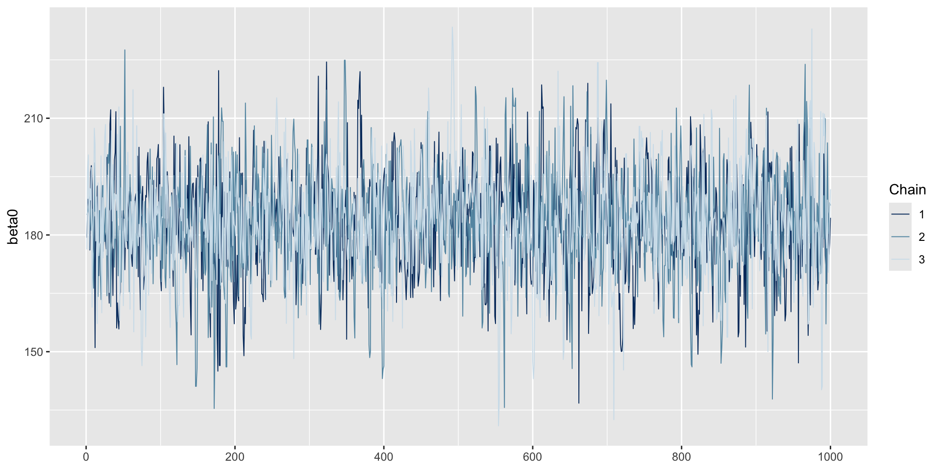
Bayesian full model using blavaan
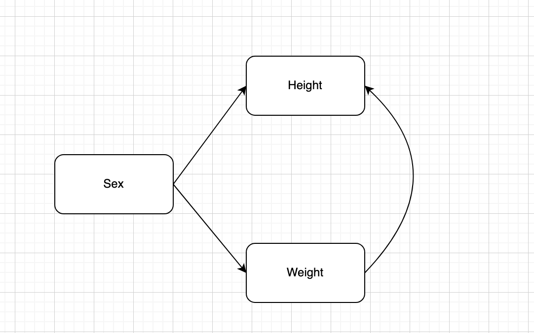
Bayesian Full Model
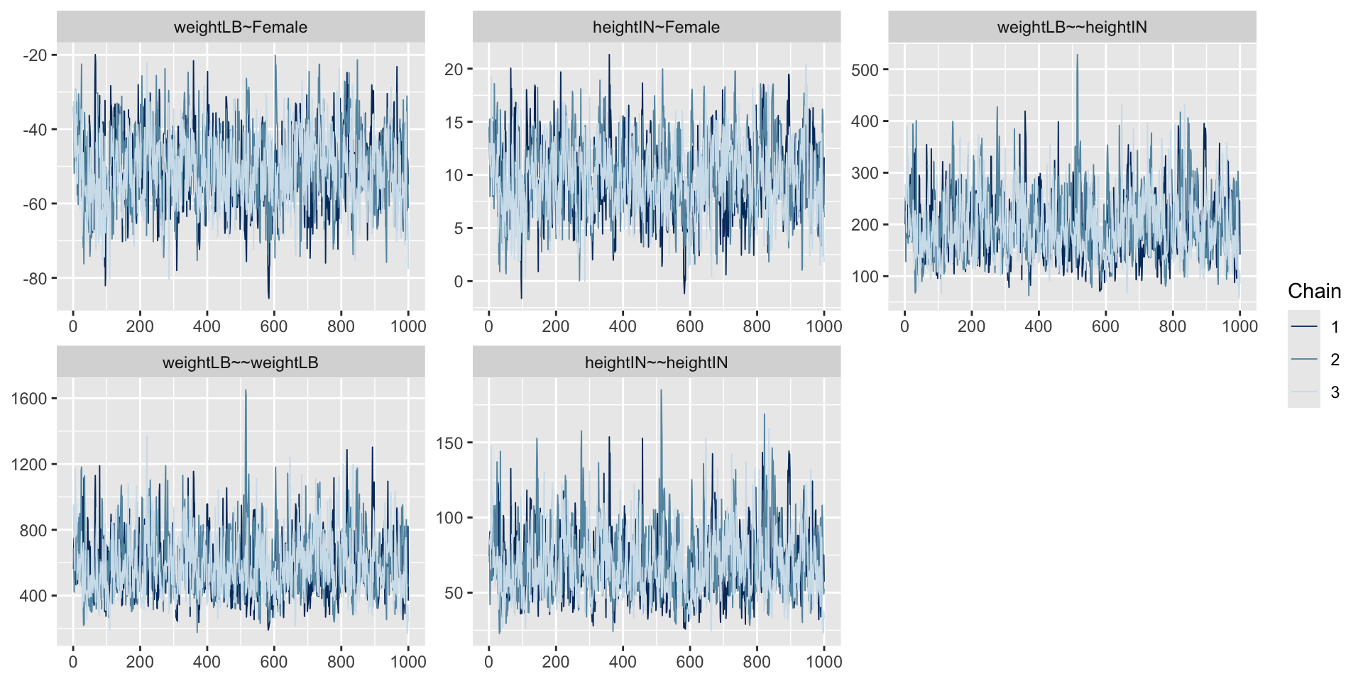
Trace Plots of Parameters
Posterior Distribution of coefficient
MLE results
       lhs op      rhs     est     se       z pvalue ci.lower ci.upper
1 weightLB  ~   Female -105.00  7.265 -14.453  0.000 -119.239  -90.761
2 heightIN  ~   Female   -8.60  2.612  -3.293  0.001  -13.718   -3.482
3 weightLB ~~ heightIN   92.34 29.602   3.119  0.002   34.322  150.358
4 weightLB ~~ weightLB  263.89 83.449   3.162  0.002  100.332  427.448
5 heightIN ~~ heightIN   34.10 10.783   3.162  0.002   12.965   55.235
6   Female ~~   Female    0.25  0.000      NA     NA    0.250    0.250
MCMC results
Summary of coefficients
blavaan 0.5.6 ended normally after 1000 iterations

  Estimator                                      BAYES
  Optimization method                             MCMC
  Number of model parameters                         5

  Number of observations                            20

  Statistic                                 MargLogLik         PPP
  Value                                             NA       0.000

Parameter Estimates:


Regressions:
                   Estimate  Post.SD pi.lower pi.upper     Rhat    Prior
  weightLB ~
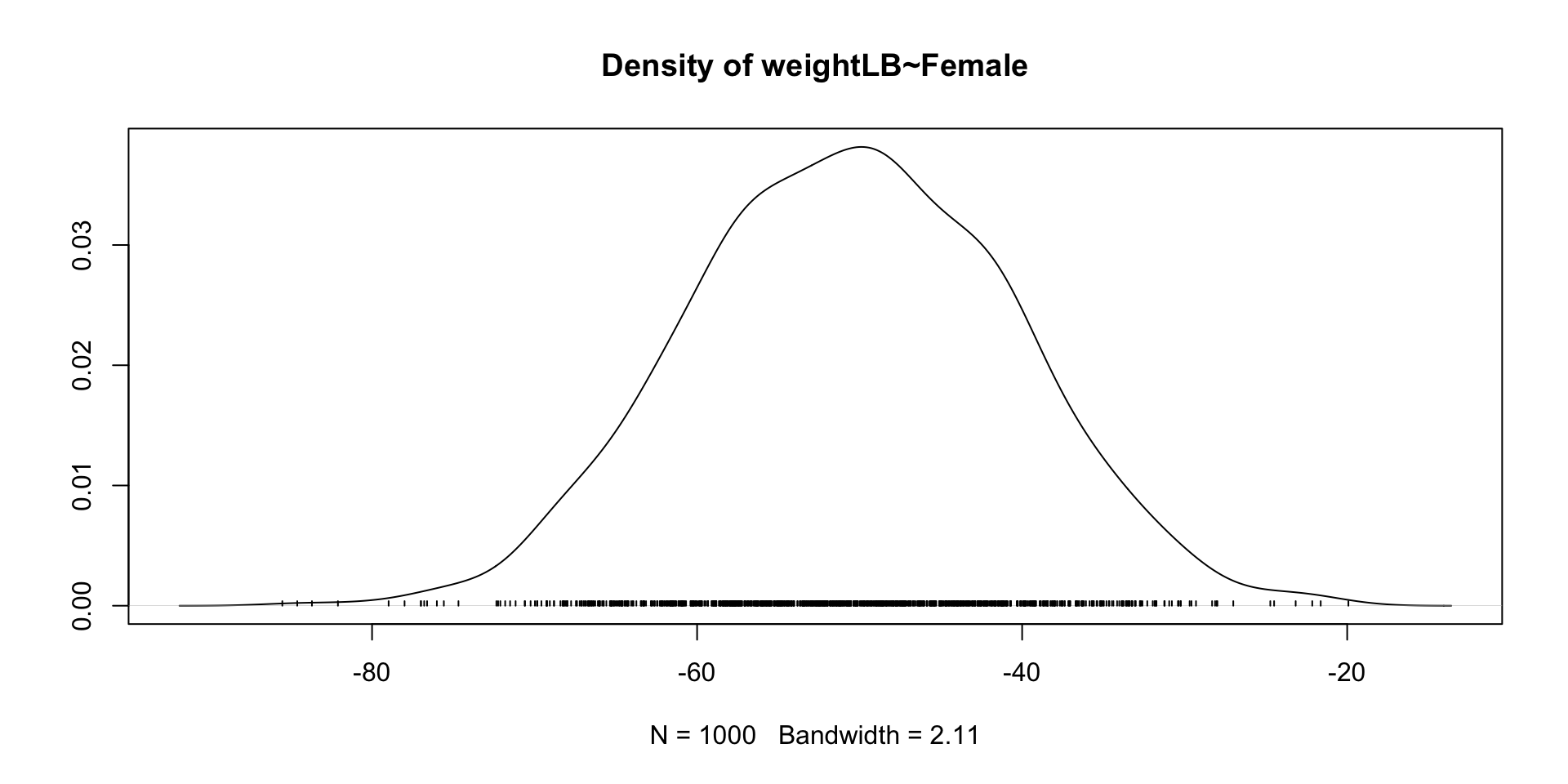
    Female          -50.561    9.872  -69.278  -31.705    1.002    normal(0,10)
  heightIN ~
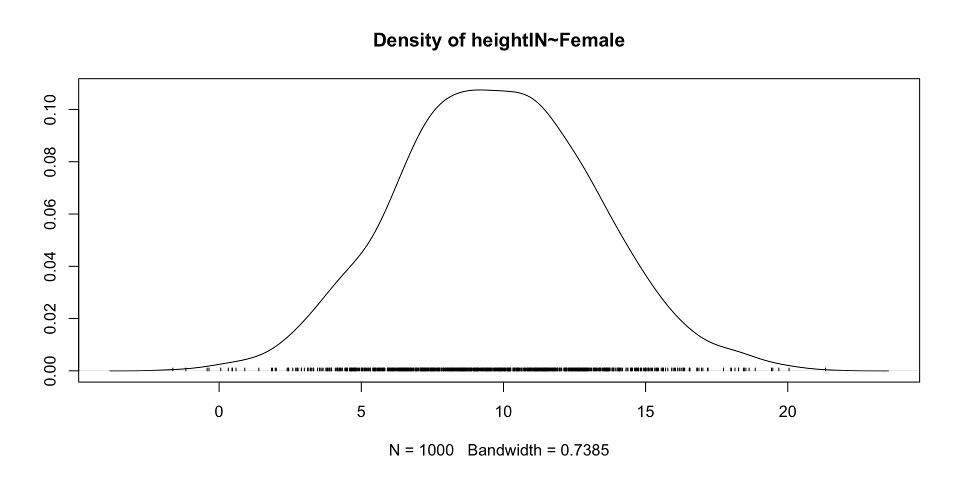
    Female            9.718    3.455    3.074   16.551    1.002    normal(0,10)

Covariances:
                   Estimate  Post.SD pi.lower pi.upper     Rhat    Prior
 .weightLB ~~
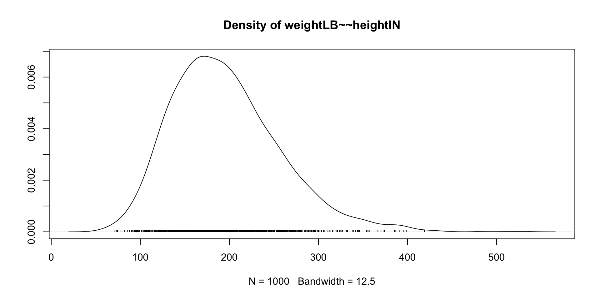
   .heightIN        196.207   60.959   99.339  339.640    1.001       beta(1,1)

Variances:
                   Estimate  Post.SD pi.lower pi.upper     Rhat    Prior
   .weightLB        582.332  181.070  296.692  997.489    1.001 gamma(1,.5)[sd]
.heightIN 69.040 21.716 35.495 119.007 1.000 gamma(1,.5)[sd]Wrapping up
Today is a quick introduction to Bayesian Concept
- Bayes’ Theorem: Fundamental theorem of Bayesian Inference
- Prior distribution: What we know about the parameter before seeing the data
- hyperparameter: parameter(s) of the prior distribution(s)
- Uninformative prior: Prior distribution that does not convey any information about the parameter
- Informative prior: Prior distribution that conveys information about the parameter
- Conjugate prior: Prior distribution that makes the posterior distribution the same family as the prior distribution
- Likelihood: What the data tell us about the parameter
- Likelihood function: Probability of the data given the parameter
- Likelihood principle: All the information about the data is contained in the likelihood function
- Likelihood is a sort of “scientific judgment” on the generation process of the data
- Posterior distribution: What we know about the parameter after seeing the data

ESRM 64503 - Lecture 11: Introduction to Bayesian
