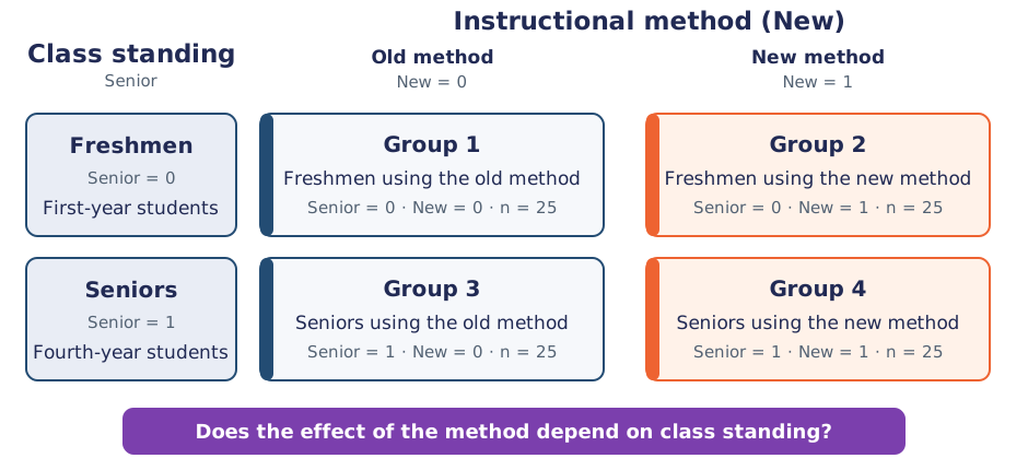
Here, Senior identifies class standing, New identifies instructional method, and Senior × New asks whether the method’s effect differs by class standing.
TipSame predictions, different interpretations
Equation 1 and Equation 2 describe the same four group means and produce the same fitted scores. What changes is the interpretation of the coefficients.
Each person’s expected (predicted) outcome is a function of his/her values on x and z (and their interaction), each measured once person
Estimated parameters are called fixed effects (here, \beta_0, \beta_1, \beta_2, and \beta_3); although they have a sampling distribution, they are not random variables
The number of fixed effects will show up in formulas as k (so k = 4 here)
Model for the Variance
e_p \sim N(0, \sigma^2_e) \rightarrow ONE residual (unexplained) deviation
e_p has a mean of 0 with some estimated constant variance \sigma^2_e, is normally distributed, is unrelated across people
Estimated parameter is the residual variance only (in the model above)
General Form of Two Models
Model for the Means (Predicted Values): The Best Guess of Estimates
Variance-Covariance Matrix of Regression Coefficients (Diagonal: variances of betas (squared standard errors of betas); Non-diagonal: residual covariances between betas)
From now on, we will think carefully about how the predictor variables enter into the model for the means rather than the scales of predictors
Why don’t people always care about the scale of predictors (centering):
Does NOT affect the amount of outcome variance account for (R^2)
Does NOT affect the outcomes values predicted by the model for the means (so long as the same predictor fixed effects are included)
Why should this matter to us?
Because the Intercept = expected outcome value when X = 0
Can end up with nonsense values for intercept if X = isn’t in the data
We will almost always need to deliberately adjust the scale of the predictor variables so that they have 0 values that could be observed in our data
Is much bigger deal in models with random effects (MLM) or GLM once interactions are included
Adjusting the Scale of Predictor Variables
For continuous (quantitative) predictors, we will make the intercept interpretable by centering:
Centering = subtract as constant from each person’s variable value so that the 0 value falls within the range of the new centered predictor variable
Typical \rightarrow Center around predictor’s mean: X_1^\prime = X_1 - \bar{X_1}
Better \rightarrow Center around meaningful constant C: X_1^\prime = X_1 - C
x <-rnorm(100, mean =1, sd =1)x_c <- x -mean(x)mean(x)mean(x_c)
[1] 1.070915
[1] 1.465494e-16
For categorical (grouping) predictors, either we or the program will make the intercept interpretable by creating a reference group:
Reference group is given a 0 value on all predictor variable created from the original group variable, such that the intercept is the expected outcome for that reference group specifically
Accomplished via “dummy coding” or “reference group coding”
For categorical predictors with more than two groups
We need to dummy coded the group variable using factor() in R
For example, I dummy coded group variable with group 1 as the reference
d1 = GroupT1 (0, 1, 0, 0) \rightarrow\beta_1 = mean difference between Treatment1 vs. Control
d2 = GroupT2 (0, 0, 1, 0) \rightarrow\beta_2 = mean difference between Treatment2 vs. Control
d3 = GroupT3 (0, 0, 0, 1) \rightarrow\beta_3 = mean difference between Treatment3 vs. Control
How does the model give us all possible group difference?
Control Mean
Treatment 1 Mean
Treatment 2 Mean
Treatment 3 Mean
\beta_0
\beta_0+\beta_1
\beta_0+\beta_2
\beta_0+\beta_3
The model (coefficients with dummy coding) directly provides 3 differences (control vs. each treatment), and indirectly provides another 3 differences (differences between treatments)
Group differences from Dummy Codes
Set J = 4 as number of groups:
The total number of group differences is J * (J-1) / 2 = 4*3/2 = 6
Control Mean
Treatment 1 Mean
Treatment 2 Mean
Treatment 3 Mean
\beta_0
\beta_0+\beta_1
\beta_0+\beta_2
\beta_0+\beta_3
All group differences
Alt Group
Ref Group
Difference
Control vs. T1
(\beta_0+\beta_1)
- \beta_0
= \beta_1
Control vs. T2
(\beta_0+\beta_2)
- \beta_0
= \beta_2
Control vs. T3
(\beta_0+\beta_3)
- \beta_0
= \beta_3
T1 vs. T2
(\beta_0+\beta_2)
-(\beta_0+\beta_1)
= \beta_2-\beta_1
T1 vs. T3
(\beta_0+\beta_3)
-(\beta_0+\beta_1)
= \beta_3-\beta_1
T2 vs. T3
(\beta_0+\beta_3)
-(\beta_0+\beta_2)
= \beta_3 - \beta_2
R Code: Estimating All Group Differences in R
library(multcomp) # install.packages("multcomp")mod_e0 <-lm(Test ~ Group, data = dataTestExperiment)summary(mod_e0)
contrast_model_matrix =matrix(c(0, 1, 0, 0, # Control vs. T10, 0, 1, 0, # Control vs. T20, 0, 0, 1, # Control vs. T30, -1, 1, 0, # T1 vs. T20, -1, 0, 1, # T1 vs. T30, 0,-1, 1# T2 vs. T3), nrow =6, byrow = T)rownames(contrast_model_matrix) <-c( "Control vs. T1", "Control vs. T2", "Control vs. T3", "T1 vs. T2", "T1 vs. T3", "T2 vs. T3" )contrast_value <-glht(mod_e0, linfct = contrast_model_matrix)summary(contrast_value)
     Simultaneous Tests for General Linear Hypotheses

Fit: lm(formula = Test ~ Group, data = dataTestExperiment)

Linear Hypotheses:
                    Estimate Std. Error t value Pr(>|t|)
Control vs. T1 == 0   7.7600     0.7586  10.229   <0.001 ***
Control vs. T2 == 0   2.1600     0.7586   2.847   0.0271 *
Control vs. T3 == 0   6.8800     0.7586   9.069   <0.001 ***
T1 vs. T2 == 0       -5.6000     0.7586  -7.382   <0.001 ***
T1 vs. T3 == 0       -0.8800     0.7586  -1.160   0.6534
T2 vs. T3 == 0        4.7200     0.7586   6.222   <0.001 ***
---
Signif. codes:  0 '***' 0.001 '**' 0.01 '*' 0.05 '.' 0.1 ' ' 1
(Adjusted p values reported -- single-step method)
What the intercept should mean to you
The model for the means will describe what happens to the predicted outcome Y “as X increases” or “as Z increases” and so forth
But you won’t know what Y is actually supposed to be unless you know where the predictor variables are starting from!
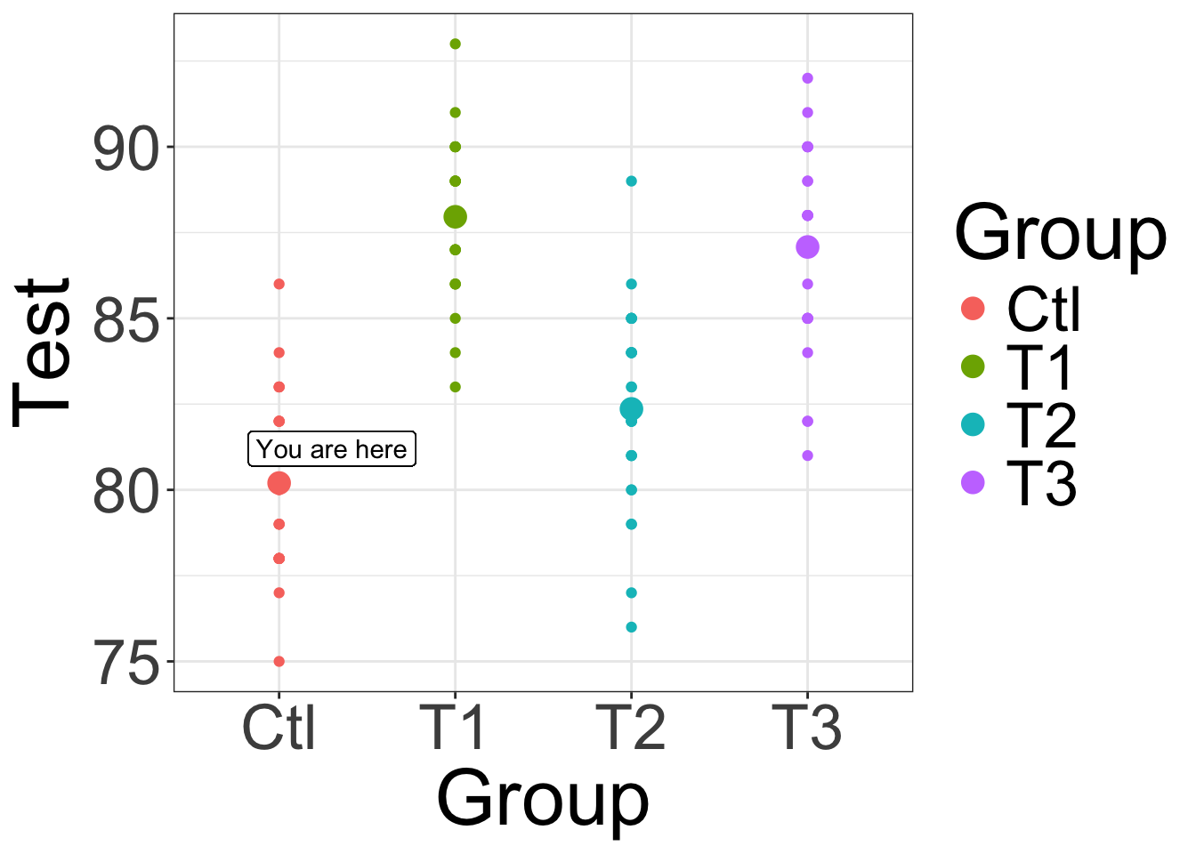
Therefore, the intercept is the “YOU ARE HERE” sign in the map of your data… so it should be somewhere in the map*!
Main Effects Within Interactions
Interaction Effects
Interaction = Moderation: the effect of a predictor depends on the value of the interacting predictor
Either predictor can be “the moderator” (interpretive distinction only)
Interaction can always be evaluated for any combination of categorical and continuous predictors, although
In “ANOVA”: By default, all possible interactions are estimated
Software does this for you; oddly enough, nonsignificant interactions usually still are kept in the model (even if only significant interactions are interpreted)
In “ANCOVA”: Continuous predictors (“covariates”) do not get to be part of interactions ➡️ make the “homogeneity of regression” assumption
There is no reason to assume this – it is a testable hypothesis!
In “Regression”: No default – effects of predictors are as you specify them
Requires most thought, but gets annoying because in regression programs you usually have to manually create the interaction as an observed variable:
e.g., XZ_interaction = centered_X * centered_Z
Simple / Conditional Main Effects in GLM with Interactions
Note
Main effects of predictors within interactions should remain in the model regardless of whether or not they are significant
Reason: the role of two-way interaction is to adjust its main effects
However, the original idea of a “main effect” no longer applied … each main effect is conditional on the interacting predictor as 0 (X_1X_2=0)
Conditional Main Effect = What it is + What modified it
Simple Main Effect = The modified value of main effect
“Conditional” main effect is a general form of “Simple” main effect:
\beta_1 is the “simple” main effect of X1 when X2 = 0
\beta_1 + \beta_3 X_2 is the “conditional” main effect of X1 depending on X2 values
\beta_2 is the “simple” main effect of X2 when X1 = 0
\beta_2 + \beta_3 X_1 is the “conditional” main effect of X2 depending on X1 values
Model-Implied Simple Main Effects: A New Example
We now move from the earlier two-by-two group example to a new example with two continuous predictors: academic motivation and final exam score.
Model-Implied Simple Main Effects: Calculations
First distinguish the general rule from a specific value calculated from that rule.
Term
Meaning
Motivation example
Conditional effect
A formula describing how the effect of a predictor changes across values of the interacting predictor.
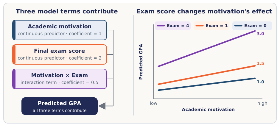
At a selected exam-score value v: b_{\text{Motiv}\mid\text{Exam}=v}=1+0.5v
Simple effect (or simple slope)
The conditional effect evaluated at one specified value of the interacting predictor.
At v=1: 1+0.5(1)=1.5
ImportantOne conditional rule, many simple effects
The conditional effect 1+0.5v generates a different simple effect at each selected exam score. The coefficient for motivation, \beta_1=1, is the simple effect specifically when Exam = 0—not an overall effect across all exam scores.
For a continuous interacting predictor, simple slope is often the clearest term. Some sources use conditional effect and simple effect interchangeably, so always report the value at which the interacting predictor is held constant.
Model-Implied Simple Main Effects: Worked Values
To compute the simple effects at selected values:
Tip
The trick is keeping track of what 0 means for every interacting predictor, which depends on the way each predictor is being represented, as determined by you, or by the software without you!
What the new coefficients mean: Predicted values stay the same.
The expected GPA is 36 when Motiv = 0 and \text{Exam}_C = 0 (that is, when Exam = 3).
The expected simple slope (effect) of Motiv is 2.5 when \text{Exam}_C = 0 (that is, when Exam = 3).
Why only two coefficients change: Re-centering changes the value called zero, so \beta_0 and \beta_1 receive new interpretations. It does not change the unit or spacing of Exam, so \beta_2 and \beta_3 remain the same.
Example: Main Effect for continuous centered predictors
Conditional main effect for Motiv depending on value of Exam:
(1 + 0.5\times\text{Exam}) or [2.5 + 0.5 \times(\text{Exam}-3)]
“Simple” main effect is 1 when Exam = 0; 2.5 when Exam = 3
Assume centering point of Exam is T, we can get the general form of simple main effect of Motivation as:
Simple slope (effect) of Motiv at \text{Exam}=v: b_{\text{Motiv}\mid\text{Exam}=v} = \beta_1 + \beta_3v
The coefficient \beta_1 is the simple slope specifically at \text{Exam}=0.
To test whether a simple slope at a selected value v differs from zero, we need both its estimate and its standard error (SE) to calculate a Wald test statistic and p-value.
Even when a simple slope is not shown as a single coefficient in the original model output, its estimate and SE are still implied by the model.
Three options can provide the simple-slope estimate and SE at a selected moderator value:
Method 1: Ask the software to give it to you using your original model
e.g., glht function in R package multicomp, ESTIMATE in SAS, TEST in SPSS, NEW in Mplus
Method 2: Re-center your predictors at the interacting value of interest (e.g., make Exam = 3 the new 0 for \text{Exam}_C) and re-estimate your model; repeat as needed for each value of interest
Method 3: Hand calculations (what the program is doing for you in option #1)
Method 3 example: At \text{Exam}=v, the estimated simple slope of Motiv is \widehat{\beta}_1 + v\widehat{\beta}_3.
Values come from “asymptotic (sampling) covariance matrix”
Variance of a sum of terms always includes covariance among them
Here, this is because what each main effect estimate could be is related to what the other main effect estimates could be
If an effect is represented by a single coefficient, its squared standard error is simply SE^2(\widehat{\beta}) = Var(\widehat{\beta}).
Unit 2: GLM Example 1
GLM via Dummy-Coding in “Regression”
# Model 1: 2 X 2 predictors with 0/1 codingmodel1 <-lm(Test ~ Senior + New + Senior * New, data = dataTestExperiment)# Alternativeformular_mod1 <-as.formula("Test ~ Senior + New + Senior * New")model1 <-lm(formular_mod1, data = dataTestExperiment)summary(model1)
Call:
lm(formula = formular_mod1, data = dataTestExperiment)

Residuals:
   Min     1Q Median     3Q    Max
 -6.36  -2.08   0.04   1.83   6.64

Coefficients:
            Estimate Std. Error t value Pr(>|t|)
(Intercept)  80.2000     0.5364 149.513  < 2e-16 ***
Senior        2.1600     0.7586   2.847  0.00539 **
New           7.7600     0.7586  10.229  < 2e-16 ***
Senior:New   -3.0400     1.0728  -2.834  0.00561 **
---
Signif. codes:  0 '***' 0.001 '**' 0.01 '*' 0.05 '.' 0.1 ' ' 1

Residual standard error: 2.682 on 96 degrees of freedom
Multiple R-squared:  0.6013,    Adjusted R-squared:  0.5888
F-statistic: 48.26 on 3 and 96 DF,  p-value: < 2.2e-16
anova(model1)
Analysis of Variance Table

Response: Test
           Df Sum Sq Mean Sq  F value    Pr(>F)
Senior      1  10.24   10.24   1.4235  0.235762
New         1 973.44  973.44 135.3253 < 2.2e-16 ***
Senior:New  1  57.76   57.76   8.0297  0.005609 **
Residuals  96 690.56    7.19
---
Signif. codes:  0 '***' 0.001 '**' 0.01 '*' 0.05 '.' 0.1 ' ' 1
Note
This ANOVA table is displaying marginal tests (F-test) for the main effects. Marginal tests are for the main effect only and are not conditional on any interacting variables.
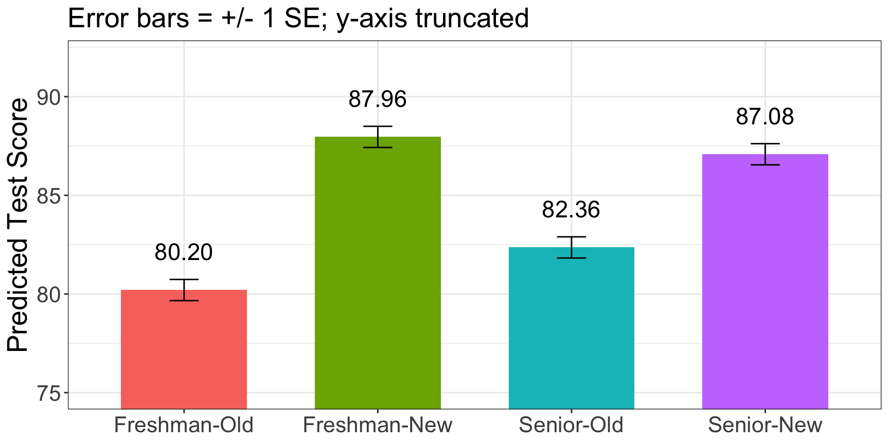
Getting estimates and standard errors of group means
Back to categorical predictors: We now return to the earlier 2 \times 2 design with class standing (Freshman/Senior) and instructional method (Old/New). The same model-implied approach allows us to estimate each group mean and its standard error.
glht() requests predicted outcomes from model for the means:
# Standard error of freshman-old group: SE(beta_0)Var_Test_1 <- Var_beta_0 <-vcov(model1)[1,1](SE_Test_1 <-sqrt(Var_Test_1))
[1] 0.5364078
# Standard error of freshman-new group: SE(beta_0+beta_1)Var_beta_0 <-vcov(model1)[1,1]Var_beta_2 <-vcov(model1)[3,3]Cov_beta_0_2 <-vcov(model1)[1,3]Var_Test_2 <- Var_beta_0 + Var_beta_2 +2*Cov_beta_0_2(SE_Test_2 <-sqrt(Var_Test_2))
[1] 0.5364078
CautionYour Homework 1 - Question 1
Copy and paste your R syntax and output that calculates the Senior-Old’s standard errors of means (use the data and model we use in class). For example, our class syntax for Freshman-New is like:
We can use glht() to automatically calculate conditional main effects and their standard errors. Or, we can manually calculate them using vcov(model) function, which represents the variance-covariance matrix of main effects.
Method 1: glht method
Using glht function to simultaneous testing for group means
Each conditional main effect is also a weighted sum of the betas, from the same model:
Senior vs. Freshmen given Old (New = 0): \mathbf{\beta_1^{Senior|New=0}=\beta_0*0+\beta_1*1+\beta_2*0+\beta_3*0}
Senior vs. Freshmen given New (New = 1): \mathbf{\beta_1^{Senior|New=1}=\beta_0*0+\beta_1*1+\beta_2*0+\beta_3*1}
New vs. Old given Freshmen (Senior = 0): \mathbf{\beta_2^{New|Senior=0}=\beta_0*0+\beta_1*0+\beta_2*1+\beta_3*0}
New vs. Old given Senior (Senior = 1): \mathbf{\beta_2^{New|Senior=1}=\beta_0*0+\beta_1*0+\beta_2*1+\beta_3*1}
Note the weight on \beta_0 is always 0: a main effect is a difference between two group means, so the intercept cancels out.
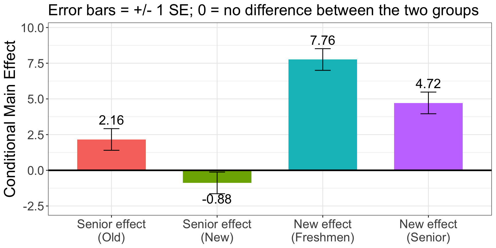
effect_model1_matrix =matrix(c(0, 1, 0, 0, # Senior vs. Freshmen | Old0, 1, 0, 1, # Senior vs. Freshmen | New0, 0, 1, 0, # New vs. Old | Freshmen0, 0, 1, 1# New vs. Old | Senior), nrow =4, byrow = T)rownames(effect_model1_matrix) <-c( "beta_Senior_New0", # Conditional Main Effect of Senior given old instruction (New = 0)"beta_Senior_New1", # Conditional Main Effect of Senior given new instruction (New = 1)"beta_New_Senior0", # Conditional Main Effect of New Instruction given Senior = 0"beta_New_Senior1") # Conditional Main Effect of New Instruction given Senior = 1effect_model1 <-glht(model1, linfct = effect_model1_matrix)summary(effect_model1)
     Simultaneous Tests for General Linear Hypotheses

Fit: lm(formula = formular_mod1, data = dataTestExperiment)

Linear Hypotheses:
                      Estimate Std. Error t value Pr(>|t|)
beta_Senior_New0 == 0   2.1600     0.7586   2.847   0.0194 *
beta_Senior_New1 == 0  -0.8800     0.7586  -1.160   0.5939
beta_New_Senior0 == 0   7.7600     0.7586  10.229   <0.001 ***
beta_New_Senior1 == 0   4.7200     0.7586   6.222   <0.001 ***
---
Signif. codes:  0 '***' 0.001 '**' 0.01 '*' 0.05 '.' 0.1 ' ' 1
(Adjusted p values reported -- single-step method)
Visualizing the four conditional main effects
Show the code for this bar plot
effect_summary <-summary(effect_model1)effect_df <-tibble(Effect =factor(names(effect_summary$test$coefficients),levels =rownames(effect_model1_matrix),labels =c("Senior effect\n(Old)", "Senior effect\n(New)","New effect\n(Freshmen)", "New effect\n(Senior)")),Estimate =as.numeric(effect_summary$test$coefficients),SE =as.numeric(effect_summary$test$sigma))ggplot(effect_df, aes(x = Effect, y = Estimate, fill = Effect)) +geom_col(width = .65) +geom_errorbar(aes(ymin = Estimate - SE, ymax = Estimate + SE), width = .15) +1geom_hline(yintercept =0, linewidth =1) +geom_text(aes(label =sprintf("%.2f", Estimate),vjust =ifelse(Estimate >0, -1.6, 2.2)), size =6) +scale_y_continuous(expand =expansion(mult =c(.15, .18))) +labs(y ="Conditional Main Effect", x =NULL,subtitle ="Error bars = +/- 1 SE; 0 = no difference between the two groups") +theme_bw() +theme(text =element_text(size =20), legend.position ="none")
1
Unlike group means, main effects are differences, so 0 is the meaningful reference line.
Method 2: vcov method
Example: Conditional main effectof Senior\mathbf{\beta_1^{Senior}} (Senior vs. Freshmen) when using the new method (New = 1)
Var_beta_1 =vcov(model1)[2,2] # squared SE of beta1Var_beta_3 =vcov(model1)[4,4] # squared SE of beta3Cov_beta_1_3 =vcov(model1)[4,2] # residual covariance of beta1 and beta3Var_beta_1_new <- Var_beta_1 + Var_beta_3 *1+2* Cov_beta_1_3 *1(SE_beta_1_new <-sqrt(Var_beta_1_new))