Lecture 05: ANOVA Comparisons and Contrasts
Experimental Design in Education
Jihong Zhang*, Ph.D
Educational Statistics and Research Methods (ESRM) Program*
University of Arkansas
2025-02-17
Class Outline
- Planned Contrast
- Example: Group Comparison - STEM vs. Non-STEM Groups
- ANOVA-style t statistics and regression-style coding in R
- Effect sizes
1 Planned Contrasts
Definition: Planned Contrasts
Pre-defined:
- Unlike post hoc tests, planned contrasts are determined before looking at the data, meaning the researcher has a specific hypothesis about which groups to compare.
- Definition: Planned contrasts are hypothesis-driven comparisons made before data collection.
Why have planned contrasts?
- They allow researchers to test specific hypotheses about group differences without the need for multiple comparisons corrections.
- They can provide more powerful tests for specific comparisons of interest.
- Example:
- In a study comparing three teaching methods (A, B, C), a planned contrast might be to compare method A against the average of methods B and C, if the researcher hypothesizes that method A will outperform the others.
Weights assigned:
- To perform a planned contrast, each group is assigned a numerical “weight” which reflects its role in the comparison, with the weights usually summing to zero.
\[ D = weights * means \]
- D: unscaled group differences given coding scheme
Example of Planned Contrasts
Imagine a study comparing the effects of three different study methods (A, B, C) on test scores.
One planned contrast might be to compare the average score of method A (considered the “experimental” method) against the combined average of methods B and C (considered the “control” conditions),
Testing the hypothesis that method A leads to significantly higher scores than the traditional methods.
\(H_0: \mu_{A} = \frac{\mu_B+\mu_C}{2}\); we also call this a complex contrast
When to use planned contrasts:
- When you have a clear theoretical basis for predicting specific differences between groups in your study.
- When you are only interested in a few specific comparisons, not all possible pairwise comparisons.
What Does Each Contrast Tell Us?
- Each contrast is a mean comparison (via t-test).
- Simple contrast (pairwise) compares two individual group means.
- Complex contrast compares a combination of group means.
- Must be theoretically justified for meaningful interpretation.
Simple vs. Complex Comparisons
- Simple Comparison: Two groups directly compared.
- Example: \(H_0: \mu_2 = \mu_3\)
- Complex Comparison: Combines means of multiple groups.
- Example: \(H_0: \frac{(\mu_1 + \mu_2)}{2} = \mu_3\)
- Example: \(H_0: \frac{(\mu_1 + \mu_2 + \mu_3)}{3} = \frac{(\mu_4 + \mu_5)}{2}\)
Note
We should not test all possible combinations of groups. Instead, justify your comparison plan before performing statistical analysis.
Today’s focus: Complex Comparisons
We performed omnibus tests in the last lecture, which provide all pairwise group comparisons (simple contrasts)
Today we focus more on complex contrasts.
- Helmert contrast: Compares each mean to the mean of subsequent groups.
- Sum (deviation) contrast: each group compared to the grand mean
- Polynomial contrast: Tests for trends in ordered data.
By default, R uses treatment contrasts: each group compared to the reference group
- Question: is “treatment contrast” a simple or complex contrast?
- G1 vs. Treatment (reference)
- G2 vs. Treatment (reference)
- ….
Orthogonal vs. Non-Orthogonal Contrasts
Orthogonal Contrasts: Independent from each other, sum of product of weights equals zero.
Non-Orthogonal Contrasts: Not independent, lead to inflated Type I error rates.
Note
Orthogonal contrasts allow clear interpretation without redundancy.
Orthogonal contrasts follow a series of group comparisons that do not overlap variances.
Orthogonal contrasts from variances: no redundancy
Helmert contrast example
- With a logical control group, a good first contrast compares all treatment groups to the one control group.
- To get each level of the IV alone, you should have one fewer contrast than your number of IV levels (3 levels = 2 contrasts)
- Once an IV level appears by itself, it shouldn’t reappear in subsequent contrasts
Example of Orthogonal Contrasts
- Contrast 1: g3 vs. (g1, g2)
![]()

- Contrast 2: g1 vs. g2
![]()

Orthogonal Planned Contrasts
- If the same exact combination of means is not found in more than one contrast, the contrasts are independent (orthogonal)
- Check this by ensuring that the product of the weights across all contrasts sums to zero
- For an orthogonal comparison, contrasts are independent of each other:
- We weight the means included on each side of the contrast
- Each contrast has weights that sum to 0
- Groups not in the contrast get a weight of 0
- Why does independence matter?
- Type I error rate is unaffected by independent (orthogonal) contrasts
- Interpretation of contrasts is cleaner because contrasts aren’t related (you’ve isolated effects)
| Group | Contrast 1 | Contrast 2 | Product |
|---|---|---|---|
| G1 | +1 | -1 | -1 |
| G2 | +1 | +1 | +1 |
| G3 | -2 | 0 | 0 |
| Sum | 0 | 0 | 0 |
Contrasts’ Independence Checking in R
Code
## Constrasts and Coding
     [,1] [,2]
[1,]    1   -1
[2,]    1    1
[3,]   -2    0
To understand if these contrasts are orthogonal, one could compute the dot product between the contrast vectors. The dot product of first and second contrast is:
\((1 * -1) + (1 * 1) + (-2 * 0) = -1 + 1 + 0 = 0\)
Since the dot product of the contrasts is equal to zero, these contrasts are indeed orthogonal.
Orthogonal contrasts have the advantage that the comparison of the means of one contrast does not affect the comparison of the means of any other contrast.
Code
## the dot-product of two contrasts should be zero
     [,1]
[1,] 0Assume we have 5 groups and we want to compare each group to the grand mean.
One one-way ANOVA may have the following contrast matrix:
Check whether the contrasts are orthogonal by calculating the cross-product of the contrast matrix.
new_code <- matrix(c(
0, 0, 0, 0,
1, 0, 0, 0,
0, 1, 0, 0,
0, 0, 1, 0,
0, 0, 0, 1
), byrow = TRUE, nrow = 5)

cat("## the cross-product of two contrasts should be zero\n")
t(new_code[,1]) %*% new_code[,2]
t(new_code[,1]) %*% new_code[,3]
t(new_code[,1]) %*% new_code[,4]
t(new_code[,2]) %*% new_code[,3]
Computing Planned Contrasts
- Formula for contrast value: \(C = c_1\mu_1 + c_2\mu_2 + \dots + c_k\mu_k\)
- Test statistic: \(t = \frac{C}{\sqrt{MSE \sum \frac{c_i^2}{n_i}}}\)
- \(MSE\): Mean Square Error from ANOVA
- \(c_i\): Contrast coefficients
- \(n_i\): Sample size per group
Planned Contrasts and Coding Scheme
The relationship between planned contrasts in ANOVA and coding in regression lies in how categorical variables are represented and interpreted in statistical models.
Both approaches aim to test specific hypotheses about group differences, but their implementation varies based on the framework:
- ANOVA focuses on partitioning variance,
- Regression interprets categorical predictors through coding schemes.
General Linear Hypothesis Testing (GLHT)
General Linear Hypothesis Testing: Planned contrast can be done using
linear regression+contrastsIn R, the
multcomppackage provides a convenient way to perform general linear hypothesis testing- Allowing us to specify custom contrasts and test them against the fitted model.
The contrast matrix can be defined manually or using built-in contrast functions in R, such as
contr.helmert,contr.sum, andcontr.treatment.Let’s look at the default contrasts plan: treatment contrasts == dummy coding
library(tidyverse)
library(kableExtra)
library(here)
# Treatment constrast
set.seed(42)
dt <- read.csv(here(
  "teaching/2025-01-13-Experiment-Design/Lecture05",
  "week5_example.csv"
))
dt$group <- factor(dt$group, levels = paste0("g", 1:5)) # order factor levels g1 to g5
## Treatment contrast matrix
constrast <- unique(model.matrix(lm(score ~ group, data = dt))) # extract unique rows of design matrix
constrast
(Intercept) groupg2 groupg3 groupg4 groupg5
1 1 0 0 0 0
29 1 1 0 0 0
57 1 0 1 0 0
85 1 0 0 1 0
113 1 0 0 0 1 Estimate Std. Error t value Pr(>|t|)
(Intercept) 4.2500000 0.4226237 10.0562268 4.227502e-18
groupg2 -1.4910714 0.5976802 -2.4947646 1.381027e-02
groupg3 -0.7053571 0.5976802 -1.1801581 2.400126e-01
groupg4 -0.3932143 0.5976802 -0.6579008 5.117222e-01
groupg5 -2.2257143 0.5976802 -3.7239217 2.871765e-04 [,1] [,2] [,3] [,4]
g1 1 0 0 0
g2 0 1 0 0
g3 0 0 1 0
g4 0 0 0 1
g5 -1 -1 -1 -1contrasts(dt$group) <- contr.sum(levels(dt$group)) # apply sum (effect) coding to group factor
mod_sum <- lm(score ~ group, data = dt) # fit model; intercept now equals grand mean
coef_table <- summary(mod_sum)$coefficients
rownames(coef_table) <- c( # rename rows for readability
"Grand Mean",
"G1 vs. Grand Mean",
"G2 vs. Grand Mean",
"G3 vs. Grand Mean",
"G4 vs. Grand Mean"
)
round(coef_table, 2) Estimate Std. Error t value Pr(>|t|)
Grand Mean 3.29 0.19 17.39 0.00
G1 vs. Grand Mean 0.96 0.38 2.55 0.01
G2 vs. Grand Mean -0.53 0.38 -1.40 0.16
G3 vs. Grand Mean 0.26 0.38 0.68 0.50
G4 vs. Grand Mean 0.57 0.38 1.51 0.13library(multcomp)
constrast <- unique(model.matrix(mod_sum)) # unique rows = one row per group
rownames(constrast) <- c( "E(G1)", "E(G2)", "E(G3)", "E(G4)", "E(G5)" ) # label rows by expected group mean
colnames(constrast) <- c( "B0", "B1", "B2", "B3", "B4" ) # label columns by beta coefficients
constrast B0 B1 B2 B3 B4
E(G1) 1 1 0 0 0
E(G2) 1 0 1 0 0
E(G3) 1 0 0 1 0
E(G4) 1 0 0 0 1
E(G5) 1 -1 -1 -1 -1
Simultaneous Tests for General Linear Hypotheses
Fit: lm(formula = score ~ group, data = dt)
Linear Hypotheses:
Estimate Std. Error t value Pr(>|t|)
E(G1) == 0 4.2500 0.4226 10.056 < 1e-05 ***
E(G2) == 0 2.7589 0.4226 6.528 < 1e-05 ***
E(G3) == 0 3.5446 0.4226 8.387 < 1e-05 ***
E(G4) == 0 3.8568 0.4226 9.126 < 1e-05 ***
E(G5) == 0 2.0243 0.4226 4.790 2.23e-05 ***
---
Signif. codes: 0 '***' 0.001 '**' 0.01 '*' 0.05 '.' 0.1 ' ' 1
(Adjusted p values reported -- single-step method)## Helmert contrast matrx
contrasts(dt$group) <- contr.helmert(levels(dt$group)) # apply Helmert coding: each group vs. mean of preceding groups
mod_helm <- lm(score ~ group, data = dt) # fit model under Helmert coding
constrast_helm <- unique(model.matrix(mod_helm)) # extract unique design matrix rows
rownames(constrast_helm) <- c( "E(G1)", "E(G2)", "E(G3)", "E(G4)", "E(G5)" )
colnames(constrast_helm) <- c( "B0", "B1", "B2", "B3", "B4" )
constrast_helm B0 B1 B2 B3 B4
E(G1) 1 -1 -1 -1 -1
E(G2) 1 1 -1 -1 -1
E(G3) 1 0 2 -1 -1
E(G4) 1 0 0 3 -1
E(G5) 1 0 0 0 4res_helm <- summary(mod_helm)$coefficients # extract coefficient table from Helmert model
rownames(res_helm) <- c( # rename rows to show what each Helmert beta represents
"Grand Mean",
"(E(G2)-E(G1))/2", # B1: G2 vs G1 mean, divided by 2
"[E(G3)-(E(G1)+E(G2))/2]/3", # B2: G3 vs average of G1-G2, divided by 3
"[E(G4)-(E(G1)+E(G2)+E(G3))/3]/4", # B3: G4 vs average of G1-G3, divided by 4
"[E(G5)-(E(G1)+E(G2)+E(G3)+E(G4))/4]/5" # B4: G5 vs average of G1-G4, divided by 5
)
res_helm Estimate Std. Error t value
Grand Mean 3.28692857 0.18900307 17.39087362
(E(G2)-E(G1))/2 -0.74553571 0.29884010 -2.49476465
[E(G3)-(E(G1)+E(G2))/2]/3 0.01339286 0.17253541 0.07762382
[E(G4)-(E(G1)+E(G2)+E(G3))/3]/4 0.08473214 0.12200096 0.69452030
[E(G5)-(E(G1)+E(G2)+E(G3)+E(G4))/4]/5 -0.31566071 0.09450154 -3.34027069
Pr(>|t|)
Grand Mean 2.818829e-36
(E(G2)-E(G1))/2 1.381027e-02
[E(G3)-(E(G1)+E(G2))/2]/3 9.382422e-01
[E(G4)-(E(G1)+E(G2)+E(G3))/3]/4 4.885495e-01
[E(G5)-(E(G1)+E(G2)+E(G3)+E(G4))/4]/5 1.082473e-03Note
Why do the Helmert coefficients have this form?
contr.helmert(5) produces weights where each column compares group \(k+1\) against the preceding \(k\) groups. The regression system for 5 groups is:
| Group | Equation |
|---|---|
| \(\mu_1\) | \(\beta_0 - \beta_1 - \beta_2 - \beta_3 - \beta_4\) |
| \(\mu_2\) | \(\beta_0 + \beta_1 - \beta_2 - \beta_3 - \beta_4\) |
| \(\mu_3\) | \(\beta_0 + 2\beta_2 - \beta_3 - \beta_4\) |
| \(\mu_4\) | \(\beta_0 + 3\beta_3 - \beta_4\) |
| \(\mu_5\) | \(\beta_0 + 4\beta_4\) |
Solving by subtraction — the earlier \(\beta\) terms cancel in the group averages:
- \(\mu_2 - \mu_1 = 2\beta_1 \Rightarrow \beta_1 = \frac{\mu_2 - \mu_1}{2}\)
- \(\mu_3 - \frac{\mu_1+\mu_2}{2} = 3\beta_2 \Rightarrow \beta_2 = \frac{\mu_3 - (\mu_1+\mu_2)/2}{3}\)
- \(\mu_4 - \frac{\mu_1+\mu_2+\mu_3}{3} = 4\beta_3 \Rightarrow \beta_3 = \frac{\mu_4 - (\mu_1+\mu_2+\mu_3)/3}{4}\)
- \(\mu_5 - \frac{\mu_1+\mu_2+\mu_3+\mu_4}{4} = 5\beta_4 \Rightarrow \beta_4 = \frac{\mu_5 - (\mu_1+\mu_2+\mu_3+\mu_4)/4}{5}\)
General pattern: \(\beta_k = \dfrac{\mu_{k+1} - \bar{\mu}_{1:k}}{k+1}\), i.e., how much group \(k+1\) exceeds the average of the preceding \(k\) groups, divided by \(k+1\).
General Linear Hypotheses
Linear Hypotheses:
Estimate
E(G1) == 0 4.250
E(G2) == 0 2.759
E(G3) == 0 3.545
E(G4) == 0 3.857
E(G5) == 0 2.024contrasts(): function to set the contrast coding for a factor variable in R. It allows you to specify how the levels of the factor should be coded for regression analysis.levels(dt$group): retrieves the levels of the factor variablegroupin the datasetdt, which are used to define the contrast coding scheme.model.matrix(): function that generates the design (or model) matrix for a linear model, based on the specified formula and data. It shows how the categorical variable is represented in the regression model according to the chosen contrast coding.
2 Example - STEM vs. Non-STEM Groups
Background
- Data: Growth mindset scores of students from five different departments (Engineering, Education, Chemistry, Political Science, Psychology).
- Hypothesis: STEM students have different growth mindset scores than non-STEM students.
- Weights assigned:
- STEM (Engineering, Chemistry): \(+\frac{1}{2}\)
- Non-STEM (Education, Political Science, Psychology): \(-\frac{1}{3}\)
- Compute contrast value and test using t-statistic.
Data Summary and Assumption Checks
Code
# Set seed for reproducibility
options(digits = 5)
summary_tbl <- dt |>
group_by(group) |>
summarise(
N = n(), # sample size per group
Mean = mean(score), # group mean
SD = sd(score), # group standard deviation
shapiro.test.p.values = shapiro.test(score)$p.value # normality test p-value (p > .05 = normal)
) |>
mutate(department = c("Engineering", "Education", "Chemistry", "Political", "Psychology")) |> # add department labels
relocate(group, department) # move group and department to first columns
summary_tbl| group | department | N | Mean | SD | shapiro.test.p.values |
|---|---|---|---|---|---|
| g1 | Engineering | 28 | 4.2500 | 3.15054 | 0.07759 |
| g2 | Education | 28 | 2.7589 | 2.19478 | 0.07605 |
| g3 | Chemistry | 28 | 3.5446 | 2.86506 | 0.00623 |
| g4 | Political | 28 | 3.8568 | 0.58325 | 0.03023 |
| g5 | Psychology | 28 | 2.0243 | 1.30911 | 0.06147 |
- Homogeneity of variance assumption: Levene’s test
Code
Levene's Test for Homogeneity of Variance (center = median)
Df F value Pr(>F)
group 4 13 5.8e-09 ***
135
---
Signif. codes: 0 '***' 0.001 '**' 0.01 '*' 0.05 '.' 0.1 ' ' 1Even though the assumption checks did not pass using the original categorical levels, we may still be interested in different group contrasts.
Stem vs. Non-Stem with Planned Contrast
For helmert and sum contrasts, the contrast matrix is pre-defined (unplanned and data-driven) and we can directly use the coefficients from the fitted model to compute the contrast value.
Code
(Intercept) group1 group2 group3 group4
3.286929 -0.745536 0.013393 0.084732 -0.315661 \[ [\beta_0 + (\beta_0 + \beta_2)] / 2 - [(\beta_0 + \beta_1) + (\beta_0 + \beta_3) + (\beta_0 + \beta_4)] / 3 \\ = \beta_2 / 2 - (\beta_1 + \beta_3 + \beta_4) /3 \]
- Expected score of reference group (Group 1, Stem): \(\beta_0\)
- Expected score of Group 2 (Non-Stem): \(\beta_0 + \beta_1\)
- Expected score of Group 3 (Stem): \(\beta_0 + \beta_2\)
- Expected score of Group 4 (Non-Stem): \(\beta_0 + \beta_3\)
- Expected score of Group 5 (Non-Stem): \(\beta_0 + \beta_4\)
Method 1: Create a new variable indicating STEM vs. Non-STEM and fit a simple linear model to test the contrast.
dt$Stem <- ifelse(dt$group %in% c("g1", "g3"), "Yes", "No") # label g1 (Engineering) and g3 (Chemistry) as STEM
dt$Stem <- factor(dt$Stem, levels = c("No", "Yes")) # set "No" as reference; "Yes" = STEM coefficient
lm(score ~ Stem, data = dt) |> summary() # simple two-group regression; sample-size weighted means
Call:
lm(formula = score ~ Stem, data = dt)
Residuals:
Min 1Q Median 3Q Max
-3.897 -1.798 0.175 1.163 6.103
Coefficients:
Estimate Std. Error t value Pr(>|t|)
(Intercept) 2.880 0.251 11.48 <2e-16 ***
StemYes 1.017 0.397 2.56 0.011 *
---
Signif. codes: 0 '***' 0.001 '**' 0.01 '*' 0.05 '.' 0.1 ' ' 1
Residual standard error: 2.3 on 138 degrees of freedom
Multiple R-squared: 0.0455, Adjusted R-squared: 0.0386
F-statistic: 6.58 on 1 and 138 DF, p-value: 0.0114Method 2: Use the multcomp package to specify the contrast directly on the fitted ANOVA model.
aov_fit <- aov(score ~ group, data = dt)
contrast <- matrix(
c(0, -1 / 3, 1 / 2, -1 / 3, -1 / 3), # g1=0 (ref, already in intercept), g2=-1/3, g3=+1/2, g4=-1/3, g5=-1/3
nrow = 1 # single-row matrix = one contrast hypothesis
)
rownames(contrast) <- "Stem vs. Non-Stem"
summary(glht(aov_fit, linfct = contrast)) # test the STEM vs. Non-STEM contrast using full ANOVA error term
Simultaneous Tests for General Linear Hypotheses
Fit: aov(formula = score ~ group, data = dt)
Linear Hypotheses:
Estimate Std. Error t value Pr(>|t|)
Stem vs. Non-Stem == 0 0.332 0.141 2.35 0.02 *
---
Signif. codes: 0 '***' 0.001 '**' 0.01 '*' 0.05 '.' 0.1 ' ' 1
(Adjusted p values reported -- single-step method)glht: general linear hypothesis test, which allows us to specify custom contrasts and test them against the fitted model.contrast: A matrix specifying the contrast of interest. In this case, we are comparing the average of the STEM groups (Group 1 and Group 3) against the average of the non-STEM groups (Group 2, Group 4, and Group 5). The weights for the STEM groups are +1/2, and the weights for the non-STEM groups are -1/3.
Why method 1 and method 2 have different p-value for t-test:
The two methods are not testing the same hypothesis, even though they’re both labeled “STEM vs Non-STEM”. That’s why the p-values differ.
Regrouping the data uses the sample sizes to weight the group means, while the contrast method uses fixed weights that do not account for sample size. This leads to different estimates of the mean difference and its standard error, resulting in different t-statistics and p-values.
Let’s break it down carefully.
🔎 What Method 1 Is Testing:
Here what we’re doing is:
Collapse the 4 (or 5) original groups into two categories
- STEM = g1, g3
- Non-STEM = the rest
Fit a simple two-group linear model.
This tests:
\[ H_0:\ \mu_{\text{STEM}} = \mu_{\text{Non-STEM}} \]
Crucially:
- The group means are weighted by sample size
- The model uses a pooled variance based on the two-category split
So the STEM mean is:
\[ \frac{n_{g1}\mu_{g1} + n_{g3}\mu_{g3}}{n_{g1} + n_{g3}} \]
and similarly for Non-STEM.
👉 This is a sample-size weighted comparison.
🔎 What Method 2 Is Testing
Here:
- Fit the full ANOVA model with all groups
- Specify a custom contrast vector
The contrast matrix:
(0, -1/3, 1/2, -1/3, -1/3)means we’re testing something like:
\[ \frac{1}{2}\mu_{g2} - \frac{1}{3}(\mu_{g1} + \mu_{g3} + \mu_{g4}) \]
(or similar depending on group ordering)
This is:
- A contrast of group means
- Using fixed mathematical weights
- NOT weighted by sample size
👉 This is an equal-weight contrast, not a sample-size weighted one.
⚠️ Why the p-values differ
There are two major reasons:
1️⃣ Different definitions of the STEM mean
Method 1:
- STEM mean = weighted by sample sizes
Method 2:
- STEM mean = equal weighting across groups
If group sizes are unequal, these are not the same number.
2️⃣ Different standard errors
Method 1:
- Variance based on 2-group model
- Degrees of freedom reflect that collapse
Method 2:
- Uses full ANOVA error term
- Standard error derived from contrast formula:
\[ SE = \sqrt{\sigma^2 \cdot c^T (X^TX)^{-1} c} \]
So even if the estimated difference were identical, the SE may differ → different t → different p.
Complex Contrast Matrix
- There are multiple “canned” contrasts: Helmert, sum (effect coding), treatment
For example, Helmert: four contrasts
Summary Statistics:
Code
dt$group <- factor(dt$group, levels = c("g1", "g2", "g3", "g4", "g5")) # reset factor level order
groups <- levels(dt$group)
cH <- contr.helmert(groups) # generate Helmert contrast matrix (4 contrasts for 5 groups)
colnames(cH) <- paste0("Ctras", 1:4) # rename columns for display clarity
summary_ctras_tbl <- cbind(summary_tbl, cH) # attach contrast weights to summary statistics table
summary_ctras_tbl group department N Mean SD shapiro.test.p.values Ctras1 Ctras2
g1 g1 Engineering 28 4.2500 3.15054 0.0775874 -1 -1
g2 g2 Education 28 2.7589 2.19478 0.0760542 1 -1
g3 g3 Chemistry 28 3.5446 2.86506 0.0062253 0 2
g4 g4 Political 28 3.8568 0.58325 0.0302312 0 0
g5 g5 Psychology 28 2.0243 1.30911 0.0614743 0 0
Ctras3 Ctras4
g1 -1 -1
g2 -1 -1
g3 -1 -1
g4 3 -1
g5 0 4Helmert contrasts are Orthogonal
Ctras1 Ctras2 Ctras3 Ctras4
0 0 0 0 Ctras1 Ctras2 Ctras3 Ctras4
Ctras1 2 0 0 0
Ctras2 0 6 0 0
Ctras3 0 0 12 0
Ctras4 0 0 0 20
Call:
lm(formula = score ~ group, data = dt)
Residuals:
Min 1Q Median 3Q Max
-4.250 -1.500 -0.269 1.214 5.991
Coefficients:
Estimate Std. Error t value Pr(>|t|)
(Intercept) 4.250 0.423 10.06 < 2e-16 ***
groupg2 -1.491 0.598 -2.49 0.01381 *
groupg3 -0.705 0.598 -1.18 0.24001
groupg4 -0.393 0.598 -0.66 0.51172
groupg5 -2.226 0.598 -3.72 0.00029 ***
---
Signif. codes: 0 '***' 0.001 '**' 0.01 '*' 0.05 '.' 0.1 ' ' 1
Residual standard error: 2.24 on 135 degrees of freedom
Multiple R-squared: 0.117, Adjusted R-squared: 0.0907
F-statistic: 4.47 on 4 and 135 DF, p-value: 0.00202Helmert, Sum, and Treatment Contrasts
The t-value for a contrast is calculated as:
\[ t = \frac{C}{\sqrt{MSE \sum \frac{c_i^2}{n_i}}} \]
where \(C\) is the contrast value, \(MSE\) is the mean square error from the ANOVA, \(c_i\) are the contrast coefficients, and \(n_i\) are the sample sizes for each group.
Thus, we can tell that:
- as the contrast value (C) increases, the t-value increases
- as the MSE increases, the t-value decreases
- as their respective sample sizes increases, the t-value decreases
Helmert Contrast
Code
[,1] [,2] [,3] [,4]
g1 -1 -1 -1 -1
g2 1 -1 -1 -1
g3 0 2 -1 -1
g4 0 0 3 -1
g5 0 0 0 4
Estimate Std. Error t value Pr(>|t|)
(Intercept) 3.286929 0.189003 17.390874 2.8188e-36
group1 -0.745536 0.298840 -2.494765 1.3810e-02
group2 0.013393 0.172535 0.077624 9.3824e-01
group3 0.084732 0.122001 0.694520 4.8855e-01
group4 -0.315661 0.094502 -3.340271 1.0825e-03[1] 3.2869 (Intercept) group1 group2 group3 group4 group
1 1 -1 -1 -1 -1 1
29 1 1 -1 -1 -1 2
57 1 0 2 -1 -1 3
85 1 0 0 3 -1 4
113 1 0 0 0 4 5 [,1] [,2] [,3] [,4]
[1,] -0.74554 0.013393 0.084732 -0.31566Treatment contrasts
For treatment contrasts, four dummy-coded variables are created to compare:
- C1: G1 (ref) vs. G2
- C2: G1 (ref) vs. G3
- C3: G1 (ref) vs. G4
- C4: G1 (ref) vs. G5
Intercept: G1’s meangroup2: G2 vs. G1group3: G3 vs. G1group4: G4 vs. G1group5: G5 vs. G1
(Intercept) groupg2 groupg3 groupg4 groupg5 group
1 1 0 0 0 0 1
29 1 1 0 0 0 2
57 1 0 1 0 0 3
85 1 0 0 1 0 4
113 1 0 0 0 1 5 Estimate Std. Error t value Pr(>|t|)
(Intercept) 4.25000 0.42262 10.0562 4.2275e-18
groupg2 -1.49107 0.59768 -2.4948 1.3810e-02
groupg3 -0.70536 0.59768 -1.1802 2.4001e-01
groupg4 -0.39321 0.59768 -0.6579 5.1172e-01
groupg5 -2.22571 0.59768 -3.7239 2.8718e-04Sum Contrasts and Effect Coding
Another type of coding is effect coding. In R, the corresponding contrast type is the so-called sum contrasts.
A detailed post about sum contrasts can be found here
With sum contrasts, the reference level is the grand mean.
- \(\frac{g1+g2+g3+g4+g5}{5}\) (grand mean) vs. g1/g2/g3/g4: the difference between mean score of g1 with grand mean across all five groups
Note
Effect coding is a method of encoding categorical variables in regression models, similar to dummy coding, but with a different interpretation of the resulting coefficients.
It is particularly useful when researchers want to compare each level of a categorical variable to the overall mean rather than to a specific reference category.
   [,1] [,2] [,3] [,4]
g1    1    0    0    0
g2    0    1    0    0
g3    0    0    1    0
g4    0    0    0    1
g5 -1 -1 -1 -1 Estimate Std. Error t value Pr(>|t|)
(Intercept) 3.28693 0.18900 17.39087 2.8188e-36
group1 0.96307 0.37801 2.54777 1.1962e-02
group2 -0.52800 0.37801 -1.39680 1.6476e-01
group3 0.25771 0.37801 0.68177 4.9655e-01
group4 0.56986 0.37801 1.50753 1.3401e-01Definition and Representation
In effect coding, categorical variables are transformed into numerical variables, typically using values of -1, 0, and 1. The key difference from dummy coding is that the reference category is represented by -1 instead of 0, and the coefficients indicate deviations from the grand mean.
For a categorical variable with k levels, effect coding requires k-1 coded variables. If we have a categorical variable X with three levels: \(A, B, C\), the effect coding scheme could be:
| Category | \(X_1\) | \(X_2\) |
|---|---|---|
| A | 1 | 0 |
| B | 0 | 1 |
| C (reference) | -1 | -1 |
The last category (\(C\)) is the reference group, coded as -1 for all indicator
- In effect coding, one level of the categorical variable (usually the last one or the one that is considered a ‘reference’ category) is coded as -1, and the others are coded as +1 or 0, suggesting their relation to the overall mean, rather than to a specific category.
Here’s how you could effect code a categorical variable with three levels (e.g., groups):
[,1] [,2]
g1 1 0
g2 0 1
g3 -1 -1This coding scheme shows that:
- Group1 (
g1) is compared to the overall effect by coding it as1in the first column and0in the second, suggesting it is above or below the overall mean. - Conversely, Group2 (
g2) is also contrasted with the overall effect. - Group3 (
g3), coded as-1in both columns, serves as the reference category against which the other two are compared.
In your regression output, the coefficients for the first two groups will show how the mean of these groups differs from the overall mean. The intercept will represent the overall mean across all groups.
Interpretation of Coefficients in effect coding
When effect coding is used in a regression model:
\[ Y = \beta_0 + \beta_1 X_1 + \beta_2 X_2 + \epsilon \]
- \(X_1\) and \(X_2\) are coded variables. They have no much meaning, but their coefficients are important
- \(\beta_0\) represents the grand mean of \(Y\) across all categories.
- \(\beta_1\) and \(\beta_2\) represent the deviation of categories \(A\) and \(B\) from the grand mean.
- The reference group (\(C\)) does not have a separate coefficient; instead, its deviation can be inferred as \(-(\beta_1 + \beta_2)\).
Code
library(ggplot2)
# Create a data frame for text labels
text_data <- data.frame(
x = rep(0.25, 3), # Repeating the same x-coordinate
y = c(0.3, 0.7, 0.9), # Different y-coordinates
label = c("C: beta[0] - beta[1] - beta[2]",
"A: beta[0] + 1*'×'*beta[1] + 0*'×'*beta[2]",
"B: beta[0] + 0*'×'*beta[1] + 1*'×'*beta[2]") # Labels
)
# Create an empty ggplot with defined limits
ggplot() +
geom_text(data = text_data, aes(x = x, y = y, label = label), parse = TRUE, size = 11) +
# Add a vertical line at x = 0.5
# geom_vline(xintercept = 0.5, color = "blue", linetype = "dashed", linewidth = 1) +
# Add two horizontal lines at y = 0.3 and y = 0.7
geom_hline(yintercept = c(0.35, 0.75, 0.95), color = "red", linetype = "solid", linewidth = 1) +
geom_hline(yintercept = 0.5, color = "grey", linetype = "solid", linewidth = 1) +
geom_text(aes(x = .25, y = .45, label = "grand mean of Y"), color = "grey", size = 11) +
# Set axis limits
xlim(0, 1) + ylim(0, 1) +
labs(y = "Y", x = "") +
# Theme adjustments
theme_minimal() +
theme(text = element_text(size = 20))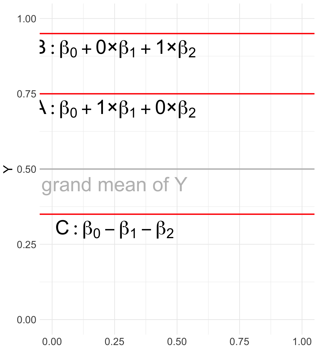
Comparison to Dummy Coding (Treatment Coding)
- Dummy Coding: Compares each category to a specific reference category (e.g., comparing A and B to C).
| Category | \(X_1\) | \(X_2\) |
|---|---|---|
| A | 1 | 0 |
| B | 0 | 1 |
| C (reference) | 0 | 0 |
- Effect Coding: Compares each category to the grand mean rather than a single reference category.
Use Cases
Effect coding is beneficial when:
- There is no natural baseline category, and comparisons to the overall mean are more meaningful.
- Researchers want to maintain sum-to-zero constraints for categorical variables in linear models.
- In ANOVA-style analyses, where main effects and interaction effects are tested under an equal-weight assumption.
Implementation in R
Effect coding can be set in R using the contr.sum function:
Exercise 1: Political Attitude and Coding Schemes
party scores
1 Democrat 4
2 Democrat 3
3 Democrat 5
4 Democrat 4
5 Democrat 4
6 Republican 6Under treatment coding, which level is the reference and how do you interpret the coefficients?
Under effect coding, what does the intercept represent and how do you interpret each group coefficient relative to the grand mean?
library(ESRM64103)
dat <- exp_political_attitude
dat$party <- factor(dat$party, levels = c("Democrat", "Republican", "Independent"))
# 1) Fit with treatment (dummy) coding
contrasts(dat$party) <- __________
fit_tr <- lm(__________)
# 2) Fit with effect (sum) coding
contrasts(dat$party) <- __________
fit_eff <- lm(__________)
# Compare ANOVA tables and coefficients
anova_tr <- anova(fit_tr)
coef_tr <- summary(fit_tr)$coef
anova_eff <- anova(fit_eff)
coef_eff <- summary(fit_eff)$coef
list(
Treatment_ANOVA = anova_tr,
Treatment_Coef = round(coef_tr, 3),
Effect_ANOVA = anova_eff,
Effect_Coef = round(coef_eff, 3)
)library(ESRM64103)
dat <- exp_political_attitude
dat$party <- factor(dat$party, levels = c("Democrat", "Republican", "Independent"))
# 1) Fit with treatment (dummy) coding
contrasts(dat$party) <- contr.treatment(3)
fit_tr <- lm(scores ~ party, data = dat)
# 2) Fit with effect (sum) coding
contrasts(dat$party) <- contr.sum(3)
fit_eff <- lm(scores ~ party, data = dat)
# Compare ANOVA tables and coefficients
anova_tr <- anova(fit_tr)
coef_tr <- summary(fit_tr)$coef
anova_eff <- anova(fit_eff)
coef_eff <- summary(fit_eff)$coef
list(
Treatment_ANOVA = anova_tr,
Treatment_Coef = round(coef_tr, 3),
Effect_ANOVA = anova_eff,
Effect_Coef = round(coef_eff, 3)
)3 Effect Sizes
What Are Effect Sizes?
- Effect size measures the magnitude of an effect beyond statistical significance.
- Put simply: a p-value is partially dependent on sample size and does not give us any insight into the strength of the relationship
- Lower p-value → can result from increasing sample size
- Provides context for interpreting practical significance.
- In scientific experiments, it is often useful to know not only whether an experiment has a statistically significant effect, but also the size (magnitude) of any observed effects.
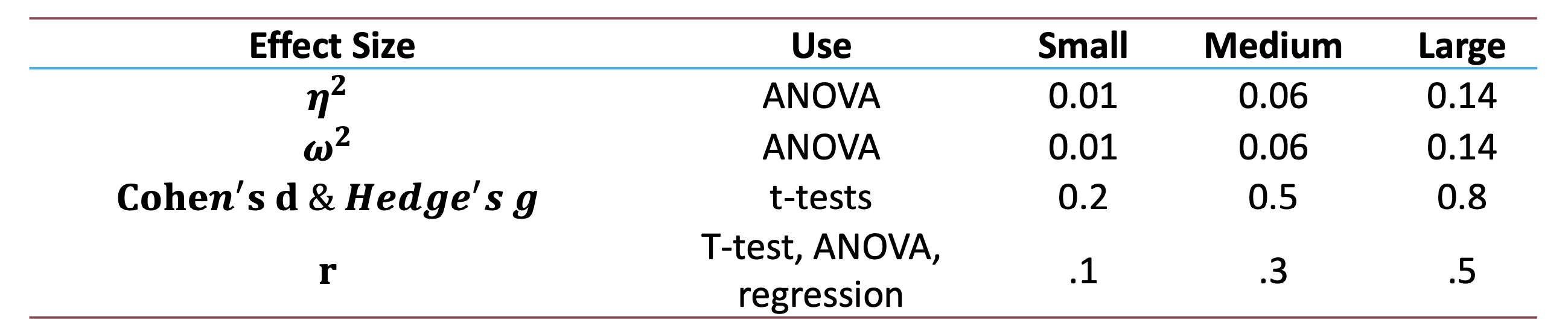
- Common measures: Eta squared (\(\eta^2\)), Omega squared (\(\omega^2\)), Cohen’s d.
Note
Many psychology journals require the reporting of effect sizes
Eta Squared
- \(\eta^2\): Proportion of total variance explained by the independent variable.
- Formula: \(\eta^2 = \frac{SS_{Model}}{SS_{Total}}\)
- Interpretation:
- Small: 0.01, Medium: 0.06, Large: 0.14
Df Sum Sq Mean Sq F value Pr(>F)
group 4 89.368 22.3420 4.4674 0.0020173
Residuals 135 675.149 5.0011 NA NAInterpretation: 11.69% of variance in the DV is due to group differences. Thus, we have a medium to large effect size.
Drawbacks of Eta Squared
- As you add more variables to the model, the proportion explained by any one variable will automatically decrease.
- This makes it hard to compare the effect of a single variable in different studies.
- Partial Eta Squared solves this problem. There, the denominator is not the total variation in Y, but the unexplained variation in Y plus the variation explained just by that IV.
- Any variation explained by other IVs is removed from the denominator.
- In a one-way ANOVA, Eta Squared and Partial Eta Squared will be equal, but this isn’t true in models with more than one independent variable (factorial ANOVA).
- Eta Squared is a biased measure of population variance explained (although it is accurate for the sample).
- It always overestimates it. This bias gets very small as sample size increases, but for small samples an unbiased effect size measure is Omega Squared.
Omega squared
- Omega Squared (\(\omega^2\)) has the same basic interpretation but uses unbiased measures of the variance components.
- Because it is an unbiased estimate of population variances, omega squared is always smaller than eta squared.
- Unbiased estimate of effect size, preferred for small samples.
- Formula: \(\omega^2 = \frac{SS_{Model} - df_{Model} \cdot MSE}{SS_{Total} + MSE}\)
- Interpretation follows \(\eta^2\) scale but slightly smaller values.
Df Sum Sq Mean Sq F value Pr(>F)
group 4 89.368 22.3420 4.4674 0.0020173
Residuals 135 675.149 5.0011 NA NA1attach(F_table)
MSE <- `Sum Sq`[2] / Df[2] # mean square error = SS_residual / df_residual
(Omega_2 <- (`Sum Sq`[1] - Df[1] * MSE) / (sum(`Sum Sq`) + MSE)) #<2> # omega^2 = (SS_model - df_model * MSE) / (SS_total + MSE)
detach(F_table)- 1
- Attach data set so that you can directly call the columns without “$”
[1] 0.090139Compute Effect Size using effectsize Package
# Effect Size for ANOVA
Parameter | Eta2 | 95% CI
-------------------------------
group | 0.12 | [0.03, 1.00]
- One-sided CIs: upper bound fixed at [1.00].# Effect Size for ANOVA
Parameter | Omega2 | 95% CI
---------------------------------
group | 0.09 | [0.01, 1.00]
- One-sided CIs: upper bound fixed at [1.00].Effect Size for Planned Contrasts
- Correlation-based effect size: \(r = \sqrt{\frac{t^2}{t^2 + df}} = \sqrt{\frac{F}{F + df}}\)
- Example: For \(t = 2.49, df = 135\): \(r = \sqrt{\frac{2.49^2}{2.49^2 + 135}} = 0.21\)
- Small to moderate effect.
            Estimate Std. Error  t value   Pr(>|t|)
(Intercept)  3.28693    0.18900 17.39087 2.8188e-36
group1       0.96307    0.37801  2.54777 1.1962e-02
group2      -0.52800    0.37801 -1.39680 1.6476e-01
group3       0.25771    0.37801  0.68177 4.9655e-01
group4 0.56986 0.37801 1.50753 1.3401e-01[1] 0.831 0.214 0.119 0.059 0.129- Shows a small to moderate positive relationship between g1 and g5.
Cohen’s d and Hedges’ g
- Used for simple mean comparisons.
- Cohen’s d formula: \(d = \frac{M_1 - M_2}{SD_{pooled}}\)
- Hedges’ g corrects for small sample bias.
- Guidelines:
- Small: 0.2, Medium: 0.5, Large: 0.8
Guidelines for Effect Size
- For our example: there is a significant effect of academic program on growth mindset scores (F(4, 135) = 4.47).
- Academic program explains 11.69% of the variance in growth mindset scores. This is a medium to large effect (\(\eta^2\) = 0.1169).
Summary
- Planned contrasts allow hypothesis-driven mean comparisons.
- Orthogonal contrasts maintain Type I error control.
- Effect sizes help interpret the importance of results.
- Combining planned contrasts with effect size measures enhances statistical analysis.

ESRM 64503