“Click here to see R code”
[1] 54.3336Experimental Design in Education
2025-04-06
Important
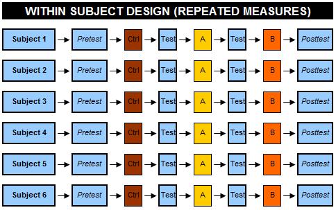
“Why subjects differ within the same group (e.g., treatment/control groups)” can be explained in RM ANOVA!
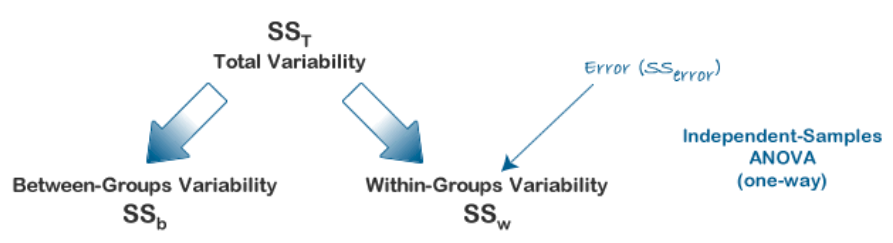
The advantage of a repeated measures ANOVA:
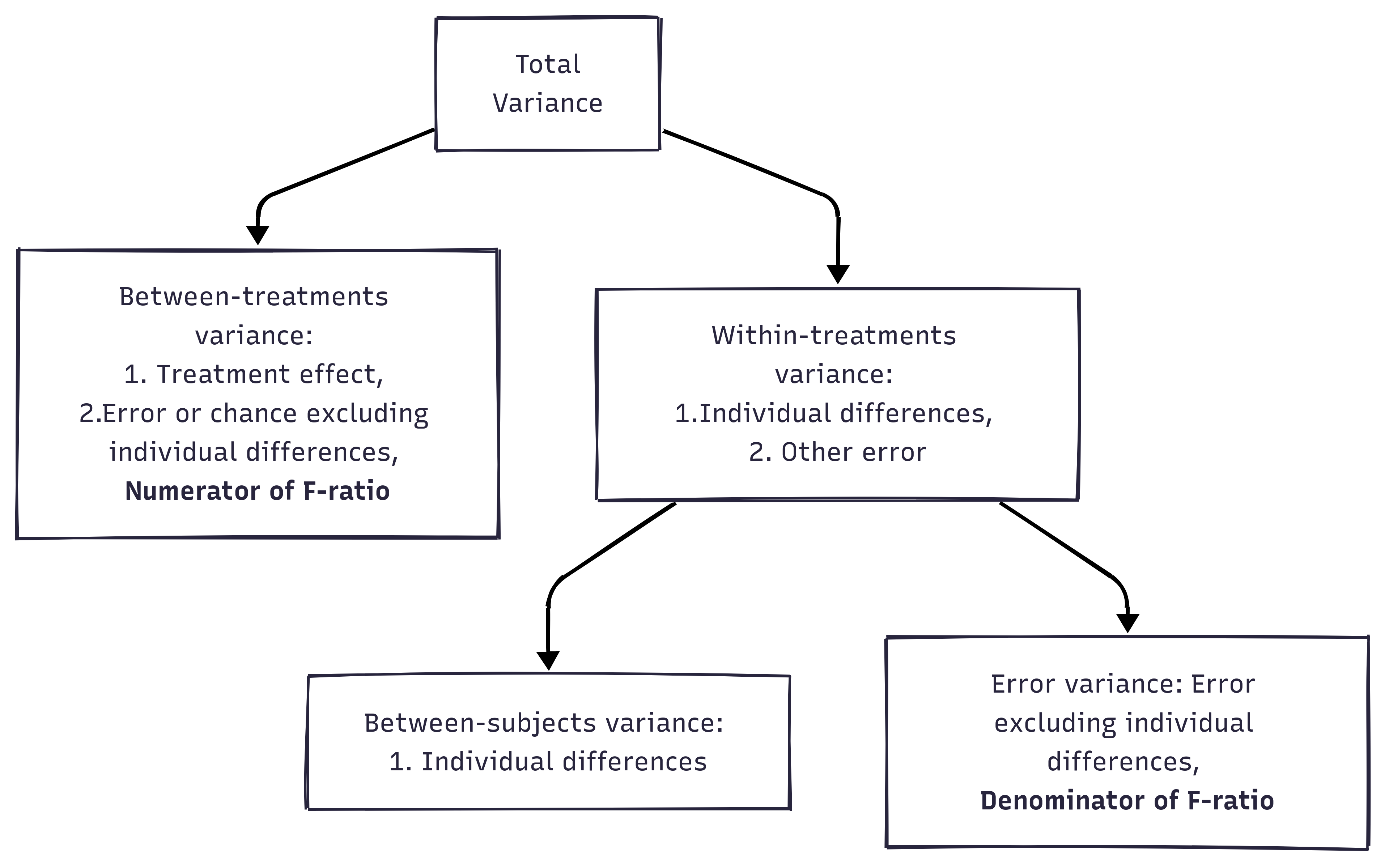
A repeated measures ANOVA calculates an F-statistic in a similar way:
 Generated by https://www.mermaidchart.com/app/projects
library(tidyverse)
library(patchwork)
set.seed(42)
n <- 8
subject_fx <- rnorm(n, 0, 2.5) # shared between-subject effect
# --- Sphericity NOT violated ---
# Residual noise is similar at every time point → equal variance of differences
no_viol_wide <- tibble(
ID = factor(1:n),
T1 = subject_fx + rnorm(n, 10, 1),
T2 = subject_fx + rnorm(n, 15, 1),
T3 = subject_fx + rnorm(n, 20, 1)
)
# --- Sphericity violated ---
# Noise is tiny at T2 but large at T3 → variance of T3-T1 >> variance of T2-T1
viol_wide <- tibble(
ID = factor(1:n),
T1 = subject_fx + rnorm(n, 10, 1),
T2 = subject_fx + rnorm(n, 15, 0.4),
T3 = subject_fx + rnorm(n, 20, 4.0)
)
to_long <- function(df) {
df |>
pivot_longer(T1:T3, names_to = "Time", values_to = "Y") |>
mutate(Time_num = as.integer(factor(Time, levels = c("T1", "T2", "T3"))))
}
no_viol <- to_long(no_viol_wide)
viol <- to_long(viol_wide)
plot_sph <- function(dat, title, shadow_col) {
means <- dat |>
group_by(Time, Time_num) |>
summarise(mean_Y = mean(Y), sd_Y = sd(Y), .groups = "drop")
ggplot(dat, aes(x = Time_num, y = Y)) +
# Shaded ribbon: mean ± 1 SD connects across time points
geom_ribbon(
data = means,
aes(x = Time_num, y = mean_Y,
ymin = mean_Y - sd_Y, ymax = mean_Y + sd_Y, group = 1),
fill = shadow_col, alpha = 0.20, inherit.aes = FALSE
) +
# Error bars at each time point to emphasise the SD width
geom_errorbar(
data = means,
aes(x = Time_num, ymin = mean_Y - sd_Y, ymax = mean_Y + sd_Y),
width = 0.12, color = shadow_col, linewidth = 1.1, inherit.aes = FALSE
) +
# Individual subject trajectories
geom_line(aes(group = ID, color = ID), alpha = 0.55, linewidth = 0.8) +
geom_point(aes(color = ID), size = 2, alpha = 0.75) +
# Group mean trajectory
geom_line(
data = means, aes(x = Time_num, y = mean_Y, group = 1),
color = "black", linewidth = 1.4, linetype = "dashed", inherit.aes = FALSE
) +
geom_point(
data = means, aes(x = Time_num, y = mean_Y),
color = "black", size = 3, inherit.aes = FALSE
) +
scale_x_continuous(breaks = 1:3, labels = c("T1", "T2", "T3")) +
scale_color_brewer(palette = "Set2") +
labs(
title = title,
subtitle = "Ribbon & bars = ±1 SD | Dashed = group mean",
x = "Time Point", y = "Outcome", color = "Subject"
) +
theme_classic(base_size = 13) +
theme(legend.position = "right")
}
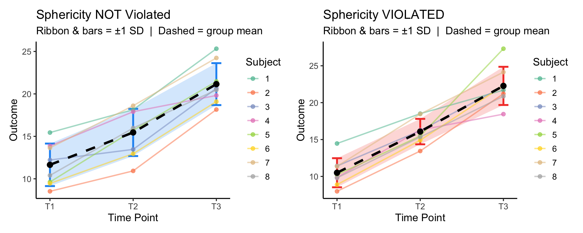
p1 <- plot_sph(no_viol, "Sphericity NOT Violated", "#2196F3")
p2 <- plot_sph(viol, "Sphericity VIOLATED", "#F44336")
p1 + p2Key intuition:
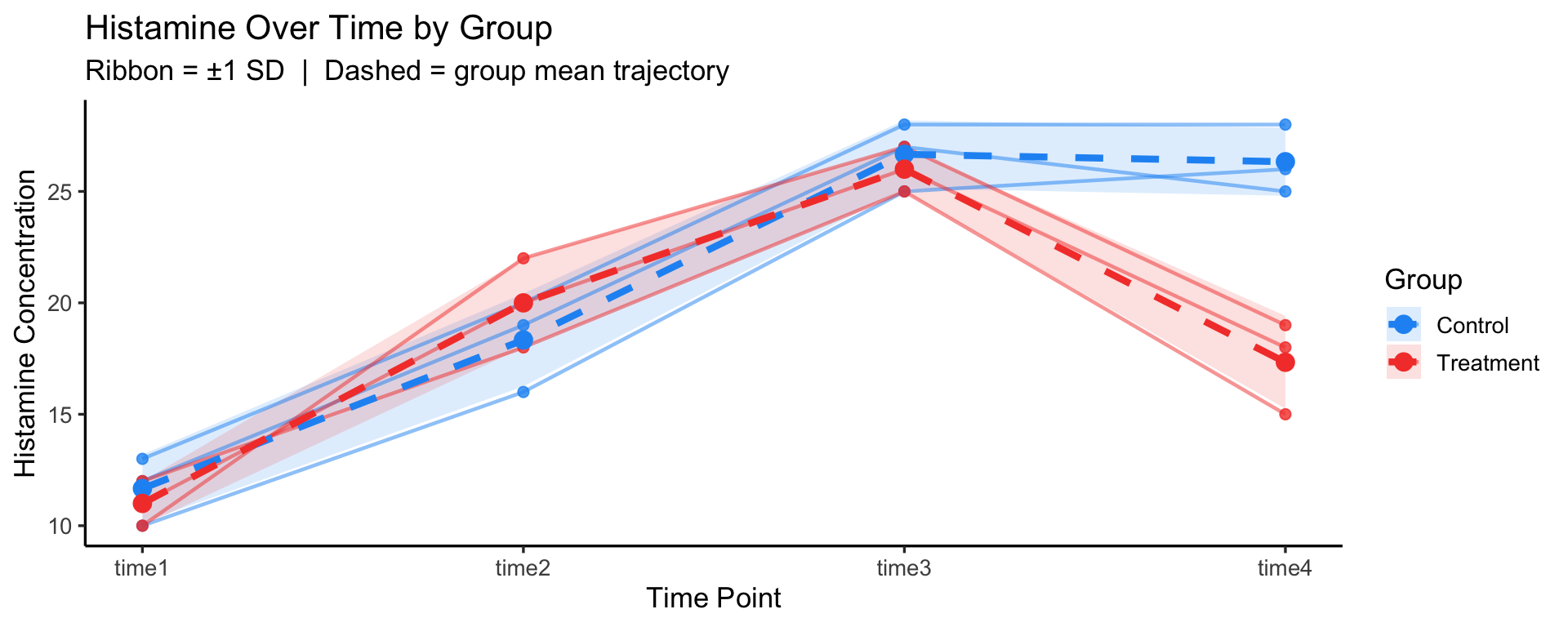
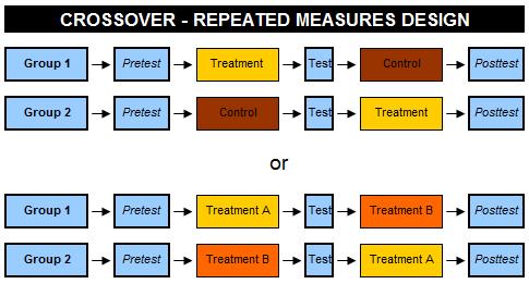
Recall the original study: six dogs, histamine measured at four time points after drug injection. Now suppose the six dogs were randomly assigned to two groups before the study began:
Discussion question: How does adding a between-subjects group factor change the analysis? What new effects can we now test?
library(tidyverse)

dat_mixed <- tribble(
  ~ID, ~Group,       ~time1, ~time2, ~time3, ~time4,
  1,   "Control",    10,     16,     25,     26,
  2,   "Control",    12,     19,     27,     25,
  3,   "Control",    13,     20,     28,     28,
  4,   "Treatment",  12,     18,     25,     15,
  5,   "Treatment",  11,     20,     26,     18,
  6,   "Treatment",  10,     22,     27,     19
) |>
  mutate(ID = factor(ID), Group = factor(Group))

dat_mixed_long <- dat_mixed |>
  pivot_longer(starts_with("time"), names_to = "Time", values_to = "Y") |>
  mutate(Time = factor(Time, levels = paste0("time", 1:4)),
         Time_num = as.integer(Time))

dat_mixed_long
# A tibble: 24 × 5
ID Group Time Y Time_num
<fct> <fct> <fct> <dbl> <int>
1 1 Control time1 10 1
2 1 Control time2 16 2
3 1 Control time3 25 3
4 1 Control time4 26 4
5 2 Control time1 12 1
6 2 Control time2 19 2
7 2 Control time3 27 3
8 2 Control time4 25 4
9 3 Control time1 13 1
10 3 Control time2 20 2
# ℹ 14 more rowslibrary(patchwork)
group_means <- dat_mixed_long |>
group_by(Group, Time, Time_num) |>
summarise(mean_Y = mean(Y), sd_Y = sd(Y), .groups = "drop")
# Individual trajectories + group mean ribbons
p_mixed <- ggplot(dat_mixed_long, aes(x = Time_num, y = Y)) +
geom_ribbon(
data = group_means,
aes(x = Time_num, y = mean_Y,
ymin = mean_Y - sd_Y, ymax = mean_Y + sd_Y,
fill = Group, group = Group),
alpha = 0.15, inherit.aes = FALSE
) +
geom_line(aes(group = ID, color = Group), alpha = 0.5, linewidth = 0.8) +
geom_point(aes(color = Group), size = 2, alpha = 0.8) +
geom_line(
data = group_means,
aes(x = Time_num, y = mean_Y, color = Group, group = Group),
linewidth = 1.5, linetype = "dashed", inherit.aes = FALSE
) +
geom_point(
data = group_means,
aes(x = Time_num, y = mean_Y, color = Group),
size = 3.5, inherit.aes = FALSE
) +
scale_x_continuous(breaks = 1:4,
labels = paste0("time", 1:4)) +
scale_color_manual(values = c(Control = "#2196F3", Treatment = "#F44336")) +
scale_fill_manual(values = c(Control = "#2196F3", Treatment = "#F44336")) +
labs(
title = "Histamine Over Time by Group",
subtitle = "Ribbon = ±1 SD | Dashed = group mean trajectory",
x = "Time Point", y = "Histamine Concentration",
color = "Group", fill = "Group"
) +
theme_classic(base_size = 13)
p_mixedBefore reading ahead — what effects should we test?
Answer
This is a Mixed Design (Split-Plot) ANOVA — it combines:
| Factor | Type | Levels |
|---|---|---|
| Group | Between-subjects | Control, Treatment |
| Time | Within-subjects | time1, time2, time3, time4 |
Three effects can now be tested:
In R:
Error: ID
          Df Sum Sq Mean Sq F value Pr(>F)
Group      1  28.17  28.167   4.306  0.107
Residuals  4  26.17   6.542

Error: ID:Time
           Df Sum Sq Mean Sq F value   Pr(>F)
Time        3  713.0  237.67  166.14 4.90e-10 ***
Group:Time  3   98.8   32.94   23.03 2.88e-05 ***
Residuals  12   17.2    1.43
---
Signif. codes:  0 '***' 0.001 '**' 0.01 '*' 0.05 '.' 0.1 ' ' 1
Group is tested against the between-subjects error (MS among dogs within groups)Time and Group:Time are tested against the within-subjects error (MS of residuals after removing dog and time effects)Looking at the plot: the two group means diverge at time4 — control dogs maintain high histamine while treatment dogs drop back. This crossing/diverging pattern is a visual cue for a potential Group × Time interaction, suggesting the drug suppresses the late-phase histamine response.
In the original study, all four time points are passive measurements after a single injection. But now suppose time3 is not a measurement — it is when the intervention (drug injection) occurs:
Discussion question: How does treating time3 as an intervention point change how we interpret the data and what comparisons matter most?
The within-subjects factor Time now has a qualitative break — the first two time points are a pre-intervention baseline and the last is a post-intervention outcome. Simply testing a main effect of Time conflates the baseline trend with the intervention effect.
A more targeted analysis would compare:
| Contrast | Formula | Question |
|---|---|---|
| Pre-trend | time3 − time1 | Was histamine already rising across the baseline period? |
| Intervention effect | time4 − time3 | Did histamine change immediately after the injection session? |
| DiD | (time4 − time3) − (time3 − time1) | Does the post-injection change exceed the natural pre-trend? |
library(tidyverse)

dat_intervention <- tribble(
  ~ID, ~time1, ~time2, ~time3, ~time4,
  1,   10,     16,     25,     26,
  2,   12,     19,     27,     25,
  3,   13,     20,     28,     28,
  4,   12,     18,     25,     15,
  5,   11,     20,     26,     18,
  6,   10,     22,     27,     19
) |>
  pivot_longer(starts_with("time"), names_to = "Time", values_to = "Y") |>
  mutate(Time = factor(Time, levels = paste0("time", 1:4)),
         Time_num = as.integer(Time),
         Phase = case_when(
           Time_num <= 2 ~ "Pre-Intervention",
           Time_num == 3 ~ "Intervention",
           Time_num == 4 ~ "Post-Intervention"
         ) |> factor(levels = c("Pre-Intervention", "Intervention", "Post-Intervention")),
         ID = factor(ID))

means_int <- dat_intervention |>
  group_by(Time, Time_num) |>
  summarise(mean_Y = mean(Y), .groups = "drop")

ggplot(dat_intervention, aes(x = Time_num, y = Y)) +
  # Shade the intervention time point
  annotate("rect", xmin = 2.5, xmax = 3.5, ymin = -Inf, ymax = Inf,
           fill = "#FF9800", alpha = 0.15) +
  annotate("text", x = 3, y = 30, label = "Intervention", color = "#E65100",
           size = 3.5, fontface = "bold") +
  geom_line(aes(group = ID, color = ID), alpha = 0.5, linewidth = 0.8) +
  geom_point(aes(color = ID), size = 2.5, alpha = 0.8) +
  geom_line(data = means_int, aes(x = Time_num, y = mean_Y, group = 1),
            color = "black", linewidth = 1.5, linetype = "dashed",
            inherit.aes = FALSE) +
  geom_point(data = means_int, aes(x = Time_num, y = mean_Y),
             color = "black", size = 3.5, inherit.aes = FALSE) +
  scale_x_continuous(breaks = 1:4, labels = paste0("time", 1:4)) +
  scale_color_brewer(palette = "Set2") +
  labs(title = "Histamine Trajectory with Intervention at time3",
       subtitle = "Shaded region = intervention session  |  Dashed = group mean",
       x = "Time Point", y = "Histamine Concentration", color = "Dog") +
  theme_classic(base_size = 13)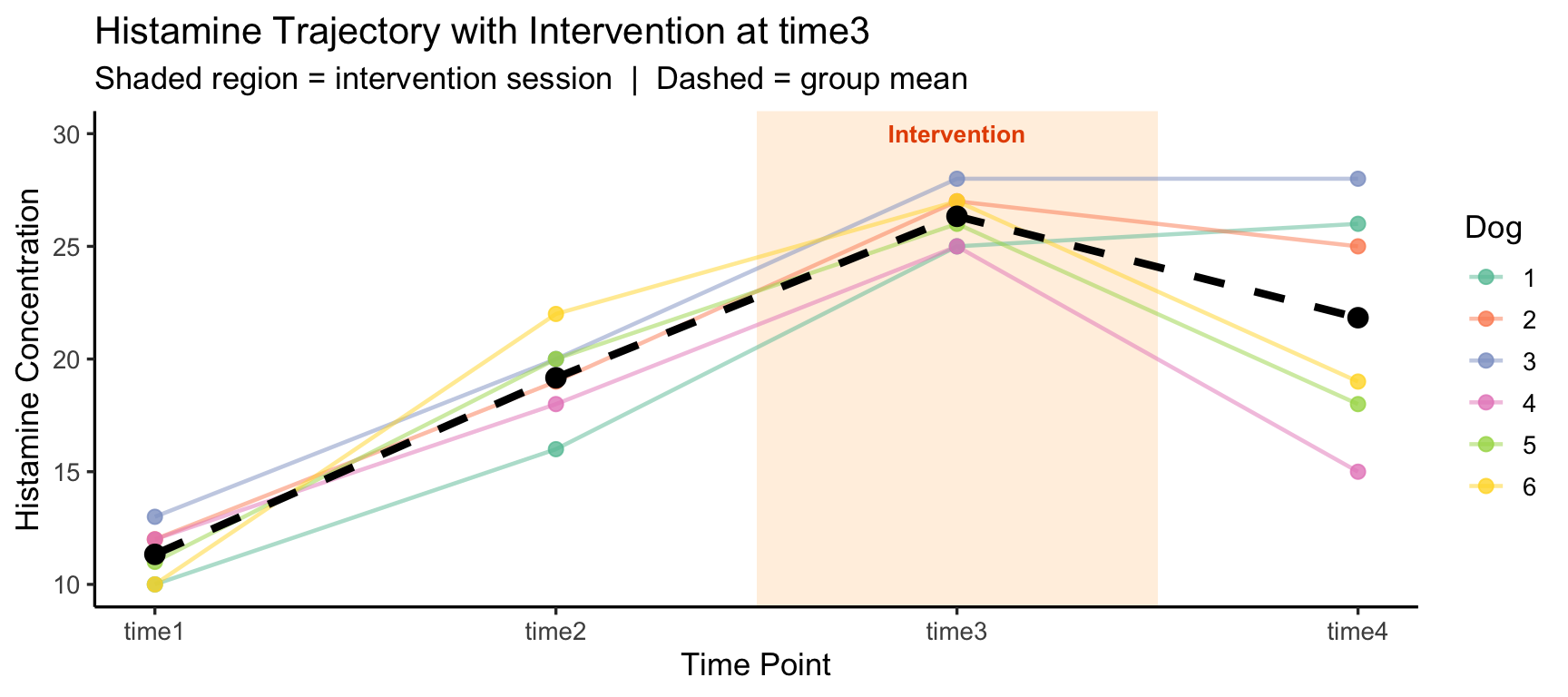
Before reading — how would you re-frame the hypothesis tests given this design?
Answer
The key shift: time3 should not be treated as just another within-subjects level — it marks a design boundary between baseline and outcome phases.
Recommended approach — planned contrasts instead of omnibus F:
library(tidyverse)

# Compute the two key contrasts per dog
contrasts_df <- dat_intervention |>
  select(ID, Time, Y) |>
  pivot_wider(names_from = Time, values_from = Y) |>
  mutate(
    pre_trend           = time3 - time1,  # baseline drift up to intervention
    intervention_effect = time4 - time3,  # post vs intervention session
    did                 = intervention_effect - pre_trend  # difference-in-differences
  )

contrasts_df |> select(ID, pre_trend, intervention_effect, did)
# A tibble: 6 × 4
ID pre_trend intervention_effect did
<fct> <dbl> <dbl> <dbl>
1 1 15 1 -14
2 2 15 -2 -17
3 3 15 0 -15
4 4 13 -10 -23
5 5 15 -8 -23
6 6 17 -8 -25Test 1 — Is the pre-intervention trend significantly different from zero?
    One Sample t-test

data:  contrasts_df$pre_trend
t = 29.047, df = 5, p-value = 9.063e-07
alternative hypothesis: true mean is not equal to 0
95 percent confidence interval:
 13.67256 16.32744
sample estimates:
mean of x
       15
Test 2 — Is there a significant intervention effect (time4 vs time3)?
    One Sample t-test

data:  contrasts_df$intervention_effect
t = -2.3342, df = 5, p-value = 0.06686
alternative hypothesis: true mean is not equal to 0
95 percent confidence interval:
 -9.4557369  0.4557369
sample estimates:
mean of x
     -4.5
Test 3 — Difference-in-differences: does the intervention effect exceed the pre-trend?
    One Sample t-test

data:  contrasts_df$did
t = -10.115, df = 5, p-value = 0.0001618
alternative hypothesis: true mean is not equal to 0
95 percent confidence interval:
 -24.45574 -14.54426
sample estimates:
mean of x
    -19.5
Visualise the contrasts per dog:
contrasts_df |>
  select(ID, pre_trend, intervention_effect, did) |>
  pivot_longer(-ID, names_to = "Contrast", values_to = "Value") |>
  mutate(Contrast = factor(Contrast,
    levels = c("pre_trend", "intervention_effect", "did"),
    labels = c("Pre-trend\n(time3 − time1)",
               "Intervention effect\n(time4 − time3)",
               "DiD\n(effect − trend)"))) |>
  ggplot(aes(x = Contrast, y = Value, color = ID, group = ID)) +
  geom_hline(yintercept = 0, linetype = "dashed", color = "grey50") +
  geom_line(alpha = 0.4, linewidth = 0.8) +
  geom_point(size = 3) +
  stat_summary(aes(group = 1), fun = mean, geom = "point",
               shape = 18, size = 5, color = "black") +
  stat_summary(aes(group = 1), fun = mean, geom = "line",
               linewidth = 1.2, color = "black", linetype = "dashed") +
  scale_color_brewer(palette = "Set2") +
  labs(title = "Planned Contrasts per Dog",
       subtitle = "Diamond = group mean  |  Dashed line at zero = no effect",
       x = NULL, y = "Contrast Value", color = "Dog") +
  theme_classic(base_size = 13)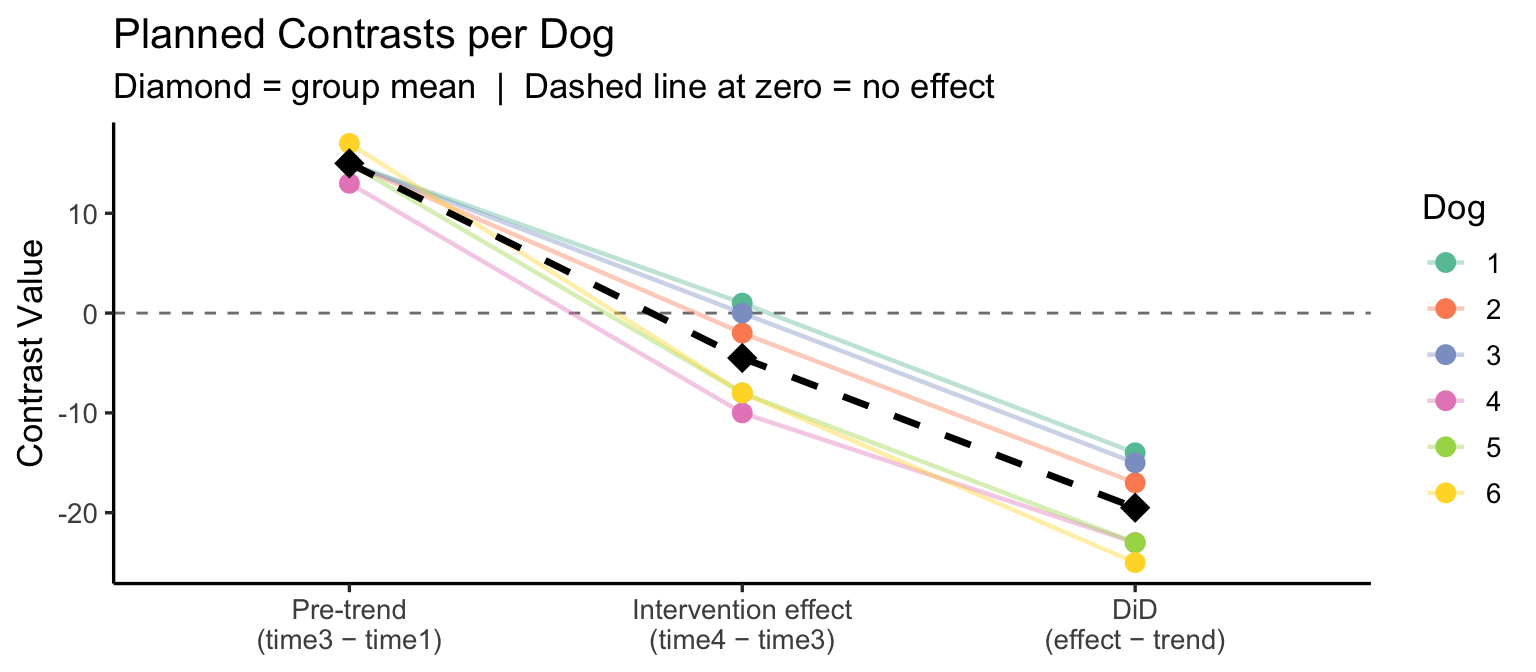
Interpretation: