Educational Statistics and Research Methods (ESRM) Program*
University of Arkansas
Published
October 9, 2024
Modified
October 11, 2024
0.1 Today’s Class
Today's Class
Multivaraite regression via path model
Model modification
Comparing and contrasting path analysis
Differences in model fit measures
How to interpret the results of path model
library(ESRM64503)library(kableExtra)library(tidyverse)library(DescTools) # Desc() allows you to quick screen datalibrary(lavaan) # Desc() allows you to quick screen data# options(digits = 3)head(dataMath)
  id hsl cc use msc mas mse perf female
1  1  NA  9  44  55  39  NA   14      1
2  2   3  2  77  70  42  71   12      0
3  3  NA 12  64  52  31  NA   NA      1
4  4   6 20  71  65  39  84   19      0
5  5   2 15  48  19   2  60   12      0
6  6  NA 15  61  62  42  87   18      0
dim(dataMath)
[1] 350 9
1 Path Analysis
Previous models considered correlations among observed variables (perf and use). These models may be limited in answering more complex research questions: whether A is a mediator between B and C
Path analysis: Multivariate Linear Models where Outcomes can be also Predictors
Path analysis details:
Model identification
Modeling workflow
Example Analyses
1.1 Today’s Example Data
Data are simulated based on the results reported in:
Sample of 350 undergraduates (229 women, 121 men)
In simulation, 10% of variables were missing (using missing completely at random mechanism).
Dictionary
Prior Experience at High School Level (HSL)
Prior Experience at College Level (CC)
Perceived Usefulness of Mathematics (USE)
Math Self-Concept (MSC)
Math Anxiety (MAS)
Math Self-Efficacy (MSE)
Math Performance (PERF)
Female (sex variable: 0 = male; 1 = female)
1.2 Multivariate Linear Regression Path Diagram
1.3 The Big Picture
Path analysis is a multivariate statistical method that, when using an identity link, assumes the variables in an analysis are multivariate normally distributed
Mean vectors
Covariance matrices
By specifying simultaneous regression equations (the core of path models), a very specific covariance matrix is implied
This is where things deviate from our familiar R matrix
Like multivariate models, the key to path analysis is finding an approximation to the unstructured (saturated) covariance matrix
With fewer parameters, if possible
The art to path analysis is in specifying models that blend theory and statistical evidence to produce valid, generalizable results
1.4 Types of Variables in Path Model
Endogenous variable(s): variables whose variability is explained by one or more variables in a model
In linear regression, the dependent variable is the only endogenous variable in an analysis
Mathematics Performance (PERF) and Mathematics Usefulness (USE)
Exogenous variable(s): variables whose variability is not explained by any variables in a model
In linear regression, the independent variable(s) are the exogenous variables in the analysis
Female (F)
1.5 Procedure of Path Analysis Steps
1.6 Identification of Path Models
Model identification is necessary for statistical models to have “meaningful” results
For path models, identification can be very difficult
Because of their unique structure, path models must have identification in two ways:
“Globally” – so that the total number of parameters does not exceed the total number of means, variances, and covariances of the endogenous and exogenous variables
“Locally” – so that each individual equation is identified
Model identification is guaranteed if a model is both “globally” and “locally” identified
1.7 Global Identification: “T-rule”
A necessary but not sufficient condition for a path models is that of having equal to or fewer model parameters than there are “distributional parameters”
Distributional parameters: As the path models we discuss assume the multivariate normal distribution, we have two matrices of parameters
The mean vector
The covariance matrix
For the MVN, the so-called T-rule states that a model must have equal to or fewer parameters than the unique elements of the covariance matrix of all endogenous and exogenous variables (the sum of all variables in the analysis)
Let s = p+q, the total of all endogenous (p) and exogenous (q) variables
Then the total unique elements are $
1.8 More on the “T-rule”
The classical definition of the “T-rule” counts the following entities as model parameters:
Direct effects (regression slopes)
Residual variances
Residual covariances
Exogenous variances
Exogenous covariances
Missing from this list are:
The set of exogenous variable means
The set of intercepts for endogenous variables
Each of the missing entities are part of the likelihood function, but are considered “saturated” so no additional parameters can be added (all parameters are estimated)
These do not enter into the equation for the covariance matrix of the endogenous and exogenous variables
1.9 T-rule Identification Status
Just-identified: number of observed covariances = number of model parameters
Necessary for identification, but no model fit indices available
Over-identified: number of observed covariances > number of model parameters
Necessary for identification; model fit indices available
Under-identified: number of observed covariances < number of model parameters
Model is NOT IDENTIFIED: No results available
1.10 Our Destination: Overall Path Model
Based on the theory described in the introduction to Pajares and Miller (1994), the following model was hypothesized – use this diagram to build your knowledge of path models
Pajares, Frank, and M. David Miller. 1994. “Role of Self-Efficacy and Self-Concept Beliefs in Mathematical Problem Solving: A Path Analysis.”Journal of Educational Psychology 86 (2): 193–203. https://doi.org/10.1037/0022-0663.86.2.193.
1.11 Overall Path Model: How to Inspect
1.12 Path Model Setup - Questions for the Analysis
How many variables are in our model? s = 7
Gender, HSL, CC, MSC, MSE, PERF, and USE
How many variables are endogenous? p = 6
HSL, CC, MSC, MSE, PERF and USE
How many variables are exogenous? q = 1
Gender
Is the model recursive or non-recursive?
Recursive – no feedback loops present
1.13 Path Model Setup – Questions for the Analysis
Is the model identified?
Check the t-rule first
How many covariance terms are there in the all-variable matrix?
\frac{7*(7+1)}{2} = 28
How many model parameters are to be estimated?
12 direct paths
6 residual variances (only endogenous variables have resid. var.)
1 variance of the exogenous variable
6 endogenous variance intercepts
Not relevant for T-rule identification, but counted in R matrix
28 (total variances/covariances) > (12 + 6 + 1) parameters, thus this model is over-identified
We can use R to run analysis
1.14 Overall Hypothesized Path Model: Equation Form
The path model from can be re-expressed in the following 6 endogenous variable regression equations:
Before we interpret the estimation result, we need to assess the fit of a multivariate linear model to the data, in an absolute sense
If a model does not fit the data:
Parameter estimates may be biased
Standard errors of estimates may be biased
Inferences made from the model may be wrong
If the saturated model fit is wrong, then the LRTs will be inaccurate
Not all “good-fitting” models are useful…
…model fit just allows you to talk about your model…there may be nothing of significance (statistically or practically) in your results, though
1.19 Global measures of Model fit
Root Mean Square Error of Approximation (RMSEA)
Likelihood ratio test
User model versus the saturated model: Testing if your model fits as well as the saturated model
The saturated model versue the baseline model: Testing whether any variables have non-zero covariances (significant correlations)
User model versus baseline model
CFI (the comparative fit index)
TLI (the Tucker–Lewis index)
Log-likelihood and Information Criteria
Standardized Root Mean Square Residual (SRMR)
How far off a model’s correlations are from the saturated model correlations
1.20 Model Fit Statistics: Example
summary(model01.fit, fit.measures =TRUE)
1Model Test User Model: Standard Scaled Test Statistic 58.89658.913 Degrees of freedom 99 P-value (Chi-square) 0.0000.000 Scaling correction factor 1.000 Yuan-Bentler correction (Mplus variant) 2Model Test Baseline Model: Test statistic 619.926629.882 Degrees of freedom 2121 P-value 0.0000.000 Scaling correction factor 0.9843Root Mean Square Error of Approximation: RMSEA 0.1260.12690 Percent confidence interval - lower 0.0960.09690 Percent confidence interval - upper 0.1570.157 P-value H_0: RMSEA <=0.0500.0000.000 P-value H_0: RMSEA >=0.0800.9940.9944User Model versus Baseline Model: Comparative Fit Index (CFI) 0.9170.918 Tucker-Lewis Index (TLI) 0.8060.809 Robust Comparative Fit Index (CFI) 0.918 Robust Tucker-Lewis Index (TLI) 0.809Loglikelihood and Information Criteria: Loglikelihood user model (H0) -5889.496-5889.496 Scaling correction factor 0.965for the MLR correction Loglikelihood unrestricted model (H1) -5860.048-5860.048 Scaling correction factor 0.975for the MLR correction Akaike (AIC) 11826.99211826.992Bayesian (BIC) 11919.58311919.583 Sample-size adjusted Bayesian (SABIC) 11843.44611843.446
1
This is a likelihood ratio (deviance) test comparing our model (H_0) with the saturated model – the saturated model fits much better (\chi^2(\Delta df = 9) = 58.896, p < .001)
2
This is a likelihood ratio (deviance) test comparing the baseline model with the saturated model
3
The RMSEA estimate is 0.126. Good fit is considered 0.05 or less.
4
The CFI estimate is .917 and the TLI is .806. Good fit is considered 0.95 or higher.
Based on the model fit statistics, we can conclude that our model does not do a good job of approximating the covariance matrix – so we cannot make inferences with these results (biased standard errors and effects may occur)
1.21 Model Modification Method 1: Check Residual Covariance
Now that we have concluded that our model fit is poor we must modify the model to make the fit better
Our modifications are purely statistical – which draws into question their generalizability beyond this sample
Generally, model modification should be guided by theory
However, we can inspect the normalized residual covariance matrix (like z- scores) to see where our biggest misfit occurs
One normalized residual covariance is bigger than +/-1.96: MSC with USE and CC with Female
The largest normalized covariances suggest relationships that may be present that are not being modeled:
Add a direct effect between F and CC
Add a direct effect between MSC and USE OR Add a residual covariance between MSC and USE
1.23 Model Midification Method 2: More Help for Fit
As we used Maximum Likelihood to estimate our model, another useful feature is that of the modification indices
Modification indices (also called Score or LaGrangian Multiplier tests) that attempt to suggest the change in the log-likelihood for adding a given model parameter (larger values indicate a better fit for adding the parameter)
Now we must start over with our path model decision tree
The model is identified (now 20 parameters < 28 covariances)
Estimation converged; Standard errors look acceptable
Model fit indices:
The comparison with the saturated model suggests our model fits statistically
The RMSEA is 0.049, which indicates good fit
The CFI and TLI both indicate good fit (CFI/TLI > .90)
The SRMR also indicates good fit
Therefore, we can conclude the model adequately approximates the covariance matrix – meaning we can now inspect our model parameters…but first, let’s check our residual covariances and modification indices
Now, no modification indices are glaringly large, although some are bigger than 3.84
We discard these as our model now fits (and adding them may not be meaningful)
2.5 More on Modification Indices
Recall from our original model that we received the following modification index values for the residual covariance between MSC and USE:
MI = 41.529
EPC = 70.912
model01.mi[2, ]
   lhs op rhs     mi    epc sepc.lv sepc.all sepc.nox
31 use ~~ msc 41.517 70.912  70.912    0.386    0.386
The estimated residual covariance between MSC and USE in the modified model is: 70.249
parameterestimates(model02.fit) |>filter(lhs =="use"& op =="~~"& rhs =="msc")
  lhs op rhs    est     se     z pvalue ci.lower ci.upper
1 use ~~ msc 70.249 10.358 6.782      0   49.947   90.551
The difference in log-likelihoods is:
-2*(change) = 58.279
anova(model01.fit, model02.fit)
Scaled Chi-Squared Difference Test (method = "satorra.bentler.2001")

lavaan->lavTestLRT():
   lavaan NOTE: The "Chisq" column contains standard test statistics, not the
   robust test that should be reported per model. A robust difference test is
   a function of two standard (not robust) statistics.
            Df   AIC   BIC  Chisq Chisq diff Df diff Pr(>Chisq)
model02.fit  8 11785 11881 14.827
model01.fit  9 11827 11920 58.896     58.279       1  2.275e-14 ***
---
Signif. codes:  0 '***' 0.001 '**' 0.01 '*' 0.05 '.' 0.1 ' ' 1
The values given by the MI and EPC are approximations
        cc        use        mse        msc       perf
0.03875216 0.04124687 0.29765620 0.48535191 0.57624994
The R2 for each endogenous variable:
CC – 0.039
USE – 0.041
MSE – 0.298
MSC – 0.485
PERF – 0.576
Note how college experience and perceived usefulness both have low percentages of variance accounted for by the model
We could have increased the R2 for USE by adding the direct path between MSC and USE instead of the residual covariance
4.5 Overall Model Interpretation
High School Experience and Female are significant predictors of College Experience (\beta_{HSL, CC} = .695, p = .006 and \beta_{F, CC} = -1.662, p = .021)
Females lower than males in College Experience
More High School Experience means more College Experience
High School Experience, College Experience, and Gender are significant predictors of Math Self-Efficacy (\beta_{HSL, MSE}= 4.05, p < .001; \beta_{CC, MSE}= .383, p < .001; \beta_{F, MSE}= 3.819, p = .001)
More High School and College Experience means higher Math Self-Efficacy
Females have higher Math Self-Efficacy than Men
High School Experience, College Experience, and Math Self-Efficacy are significant predictors of Math Self-Concept (\beta_{HSL, MSC}= 2.894, p < .001; \beta_{CC, MSC}= .545, p < .001; \beta_{MSE, MSC}= .692, p < .001)
More High School and College Experience and higher Math Self-Efficacy mean higher Math Self-Concept
Higher Math Self-Efficacy means significantly higher Perceived Usefulness
Higher Math Self-Efficacy and Math Self-Concept result in higher Math Performance scores
Math Self-Concept and Perceived Usefulness have a significant residual covariance
4.6 Wrapping Up
In this lecture we discussed the basics of path analysis
Model specification/identification
Model estimation
Model fit (necessary, but not sufficient)
Model modification and re-estimation
Final model parameter interpretation
There is a lot to the analysis – but what is important to remember is the over-arching principal of multivariate analyses: covariance between variables is important
Path models imply very specific covariance structures
The validity of the results hinge upon accurately finding an approximation to the covariance matrix
---title: "Lecture 09: Path Analysis"subtitle: "Absolute Model fit and Model Interpretation"author: "Jihong Zhang*, Ph.D"institute: | Educational Statistics and Research Methods (ESRM) Program* University of Arkansasdate: "2024-10-09"date-modified: "2024-10-11"sidebar: falseexecute: echo: true warning: falseoutput-location: defaultcode-annotations: belowhighlight-style: "nord"format: uark-revealjs: scrollable: true chalkboard: true embed-resources: false code-fold: false number-sections: false footer: "ESRM 64503 - Lecture 09: Absolute Model fit and Path Analysis" slide-number: c/t tbl-colwidths: auto output-file: slides-index.html html: page-layout: full toc: true toc-depth: 2 toc-expand: true lightbox: true code-fold: false fig-align: centerfilters: - quarto - line-highlightbibliography: references.bib---## Today's Class```{=html}<div class="card shadow"> <div class="ml-3 mt-2"> <svg xmlns="http://www.w3.org/2000/svg" width="54" height="14" viewBox="0 0 54 14"> <g fill="none" fill-rule="evenodd" transform="translate(1 1)"> <circle cx="6" cy="6" r="6" fill="#FF5F56" stroke="#E0443E" stroke-width=".5"></circle> <circle cx="26" cy="6" r="6" fill="#FFBD2E" stroke="#DEA123" stroke-width=".5"></circle> <circle cx="46" cy="6" r="6" fill="#27C93F" stroke="#1AAB29" stroke-width=".5"></circle> </g> </svg> </div> <div class="card-body"> <h4 class="card-title"><b>Today's Class</b></h4> <ul> <li>Multivaraite regression via path model</li> <li>Model modification</li> <li>Comparing and contrasting path analysis</li> <ul> <li>Differences in model fit measures </li> </ul> <li>How to interpret the results of path model</li> </ul> </div></div>``````{r}#| output-location: defaultlibrary(ESRM64503)library(kableExtra)library(tidyverse)library(DescTools) # Desc() allows you to quick screen datalibrary(lavaan) # Desc() allows you to quick screen data# options(digits = 3)head(dataMath)dim(dataMath)```# Path Analysis- Previous models considered correlations among observed variables (`perf` and `use`). These models may be limited in answering more complex research questions: whether A is a mediator between B and C- Path analysis: Multivariate Linear Models where Outcomes can be also Predictors- Path analysis details: - Model identification - Modeling workflow- Example Analyses## Today's Example Data- Data are simulated based on the results reported in:- Sample of 350 undergraduates (229 women, 121 men) - In simulation, 10% of variables were missing (using missing completely at random mechanism).::: callout-tip## Dictionary1. Prior Experience at High School Level (HSL)2. Prior Experience at College Level (CC)3. Perceived Usefulness of Mathematics (USE)4. Math Self-Concept (MSC)5. Math Anxiety (MAS)6. Math Self-Efficacy (MSE)7. Math Performance (PERF)8. Female (sex variable: 0 = male; 1 = female):::## Multivariate Linear Regression Path Diagram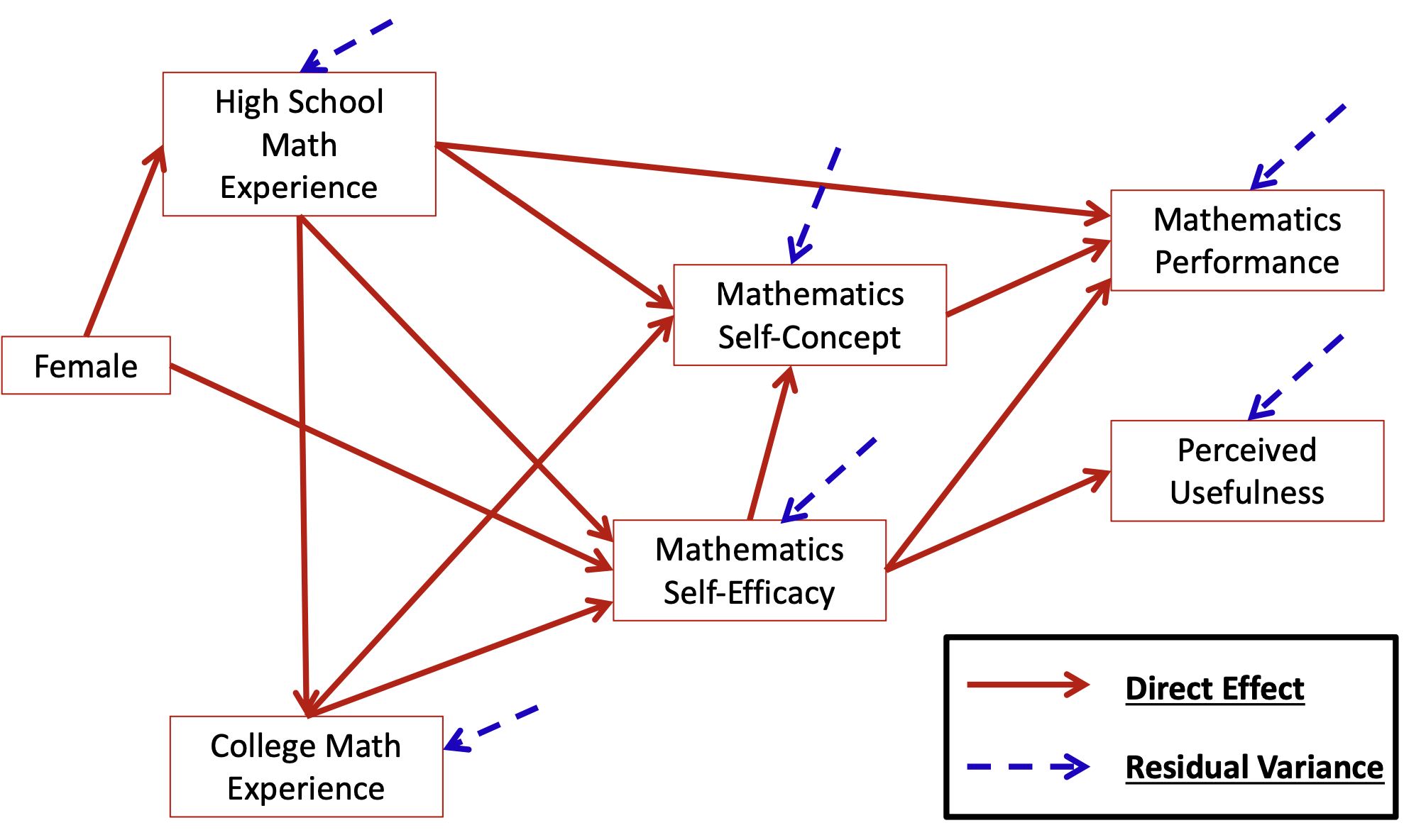{fig-align="center"}## The Big Picture1. **Path analysis** is a multivariate statistical method that, when using an identity link, assumes the variables in an analysis are multivariate normally distributed - Mean vectors - Covariance matrices2. By specifying simultaneous regression equations (the core of path models), a very specific covariance matrix is implied - This is where things deviate from our familiar R matrix3. Like multivariate models, the key to path analysis is finding an approximation to the unstructured (saturated) covariance matrix - With fewer parameters, if possible4. The art to path analysis is in specifying models that blend theory and statistical evidence to produce valid, generalizable results## Types of Variables in Path Model- **Endogenous variable(s)**: variables whose variability is explained by one or more variables in a model - In linear regression, the dependent variable is the only endogenous variable in an analysis - Mathematics Performance (PERF) and Mathematics Usefulness (USE)- **Exogenous variable(s)**: variables whose variability is not explained by any variables in a model - In linear regression, the independent variable(s) are the exogenous variables in the analysis - Female (F)## Procedure of Path Analysis Steps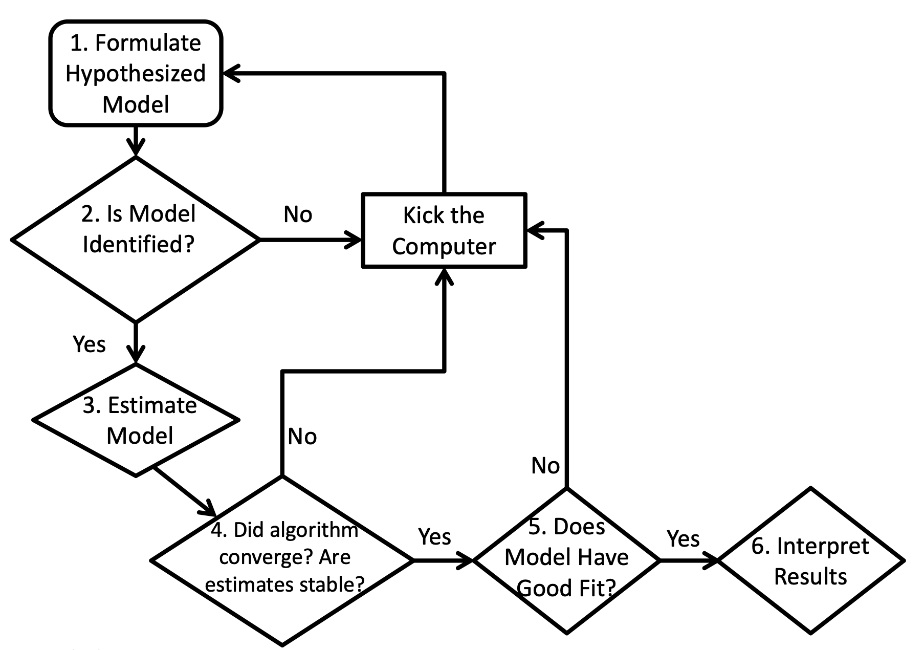{fig-align="center"}## Identification of Path Models- Model identification is necessary for statistical models to have "meaningful" results- For path models, identification can be very difficult- Because of their unique structure, path models must have identification in two ways: - "Globally" – so that the total number of parameters does not exceed the total number of means, variances, and covariances of the endogenous and exogenous variables - "Locally" – so that each individual equation is identified- Model identification is guaranteed if a model is both "globally" and "locally" identified## Global Identification: "T-rule"- A necessary but not sufficient condition for a path models is that of having equal to or fewer model parameters than there are "[distributional parameters]{.underline}"- Distributional parameters: As the path models we discuss assume the multivariate normal distribution, we have two matrices of parameters - The mean vector - The covariance matrix- For the MVN, the so-called **T-rule** states that a model must have equal to or fewer parameters than the unique elements of the covariance matrix of all endogenous and exogenous variables (the sum of all variables in the analysis) - Let $s = p+q$, the total of all endogenous (p) and exogenous (q) variables - Then the total unique elements are \$\frac{s(s+1)}{2}## More on the "T-rule"- The classical definition of the "T-rule" counts the following entities as model parameters: 1. Direct effects (regression slopes) 2. Residual variances 3. Residual covariances 4. Exogenous variances 5. Exogenous covariances- Missing from this list are: 1. The set of exogenous variable means 2. The set of intercepts for endogenous variables- Each of the missing entities are part of the likelihood function, but are considered “saturated” so no additional parameters can be added (all parameters are estimated) - These do not enter into the equation for the covariance matrix of the endogenous and exogenous variables## T-rule Identification Status- Just-identified: number of observed covariances = number of model parameters - Necessary for identification, but no model fit indices available- Over-identified: number of observed covariances \> number of model parameters - Necessary for identification; model fit indices available- Under-identified: number of observed covariances \< number of model parameters - Model is [NOT IDENTIFIED]{.underline}: No results available## Our Destination: Overall Path Model- Based on the theory described in the introduction to @pajaresRoleSelfefficacySelfconcept1994, the following model was hypothesized – use this diagram to build your knowledge of path models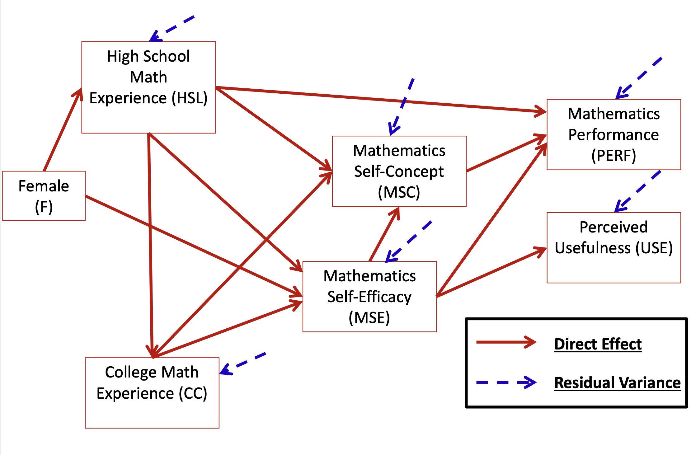{fig-align="center"}## Overall Path Model: How to Inspect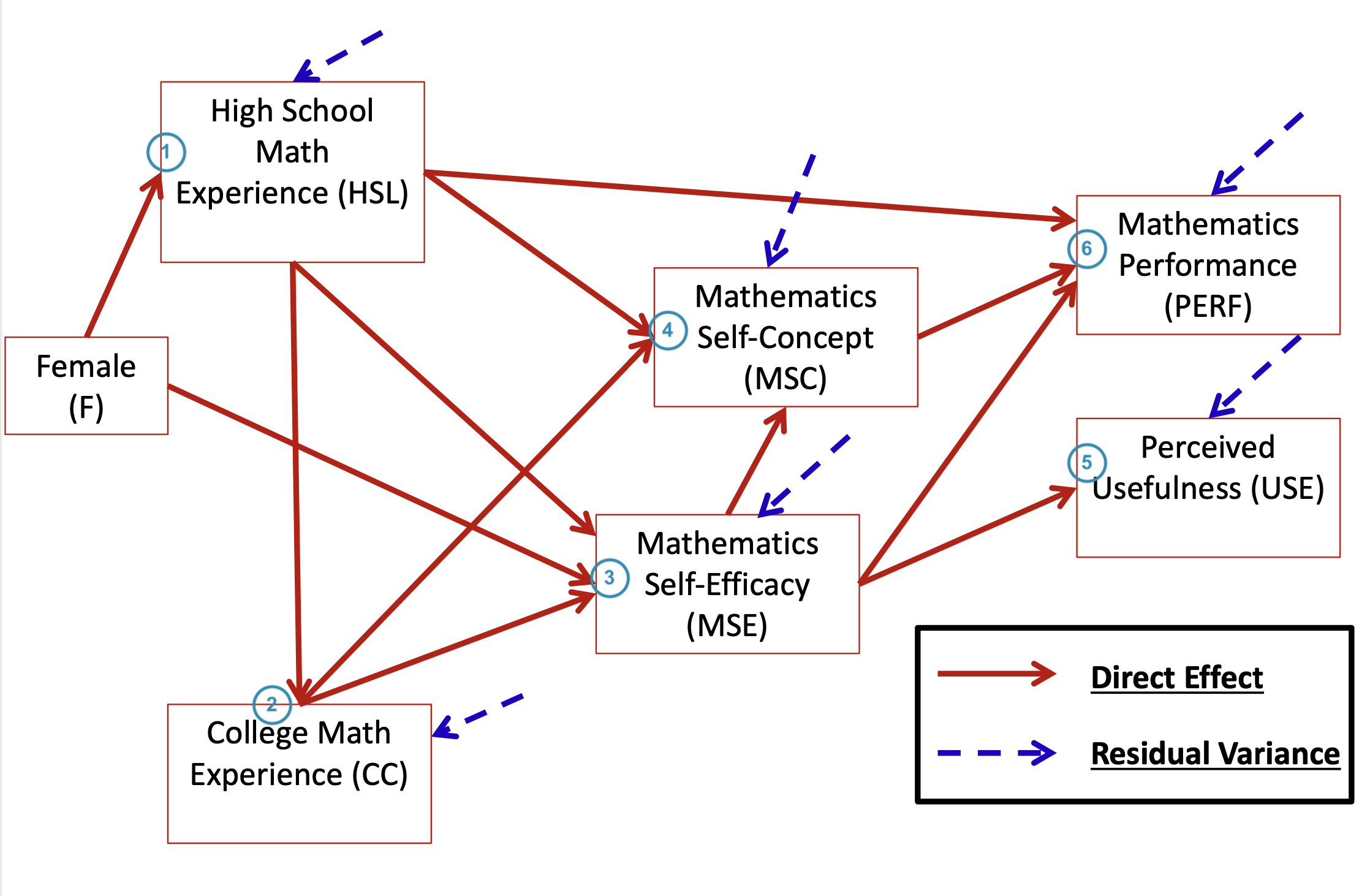{fig-align="center"}## Path Model Setup - Questions for the Analysis- How many variables are in our model? $s = 7$ - Gender, HSL, CC, MSC, MSE, PERF, and USE- How many variables are endogenous? $p = 6$ - HSL, CC, MSC, MSE, PERF and USE- How many variables are exogenous? $q = 1$ - Gender- Is the model recursive or non-recursive? - Recursive – no feedback loops present## Path Model Setup – Questions for the Analysis- Is the model identified? - Check the t-rule first - How many covariance terms are there in the all-variable matrix? - $\frac{7*(7+1)}{2} = 28$ - How many model parameters are to be estimated? - 12 direct paths - 6 residual variances (only endogenous variables have resid. var.) - 1 variance of the exogenous variable - 6 endogenous variance intercepts - Not relevant for T-rule identification, but counted in R matrix- 28 (total variances/covariances) \> (12 + 6 + 1) parameters, thus this model is over-identified - We can use R to run analysis## Overall Hypothesized Path Model: Equation Form{fig-align="center" width="1000"}- The path model from can be re-expressed in the following 6 endogenous variable regression equations:$$HSL_i = \beta_{0, HSL} + \beta_{F, HSL}F_i + e_{i, HSL}$$ {#eq-reg1}$$CC_i = \beta_{0,CC}+\beta_{HSL,CC}HSL_i + e_{i,CC}$$ {#eq-reg2}$$MSE_i = \beta_{0,MSE} + \beta_{F,MSE}F_i +\beta_{HSL,MSE}HSL_i + \beta_{CC,MSE}CC_i +e_{i,MSE}$$ {#eq-reg3}$$MSC_i = \beta_{0, MSE} + \beta_{HSL,MSC}HSL_i + \beta_{CC,MSC} CC_i + \beta_{MSE,MSC} MSE_i + e_{i,MSC}$$ {#eq-reg4}$$USE_i = \beta_{0,USE} + \beta_{MSE,USE}MSE_{i} + e_{i, USE}$$ {#eq-reg5}$$PERF_i = \beta_{0,PERF} + \beta_{HSL,PERF}HSL_{i} +\beta_{MSE,PERF}MSE_i + \beta_{MSC, PERF}MSC_{i} + e_{i,PERF}$$ {#eq-reg6}## Data Analytic Plan1. Constructed our model2. Verified it was identified using the t-rule and that it is a recursive model3. Estimate the model with R4. Check model fit## Path Model: `lavaan` syntax```{r}#model 01-----------------------------------------------------------------------model01.syntax =" #endogenous variable equationsperf ~ hsl + msc + mseuse ~ msemse ~ hsl + cc + female msc ~ mse + cc + hslcc ~ hslhsl ~ female#endogenous variable interceptsperf ~ 1use ~ 1mse ~ 1msc ~ 1cc ~ 1hsl ~ 1#endogenous variable residual variancesperf ~~ perfuse ~~ usemse ~~ msemsc ~~ msccc ~~ cc hsl ~~ hsl#endogenous variable residual covariances#none specfied in the original model so these have zeros:perf ~~ 0*use + 0*mse + 0*msc + 0*cc + 0*hsluse ~~ 0*mse + 0*msc + 0*cc + 0*hslmse ~~ 0*msc + 0*cc + 0*hslmsc ~~ 0*cc + 0*hslcc ~~ 0*hsl"```## Model Fit Evaluation- First, we check convergence: - `lavaan`'s ML algorithm converged!```{r}#estimate modelmodel01.fit =sem(model01.syntax, data=dataMath, mimic ="MPLUS", estimator ="MLR")#see if model convergedinspect(model01.fit, what="converged")```- Second, we check for abnormally large standard errors: - None too big, relative to the size of the parameter - Indicates identified mdoel```{r} parameterestimates(model01.fit) |> filter(op != "~~") ```- Third, we look at the model fit statistics.## Model Fit Statistics- Before we interpret the estimation result, we need to assess the fit of a multivariate linear model to the data, in an absolute sense- If a model does not fit the data: - Parameter estimates may be biased - Standard errors of estimates may be biased - Inferences made from the model may be wrong - If the saturated model fit is wrong, then the LRTs will be inaccurate- Not all “good-fitting” models are useful… - …model fit just allows you to talk about your model…there may be nothing of significance (statistically or practically) in your results, though## Global measures of Model fit1. Root Mean Square Error of Approximation (RMSEA)2. Likelihood ratio test - User model versus the saturated model: Testing if your model fits as well as the saturated model - The saturated model versue the baseline model: Testing whether any variables have non-zero covariances (significant correlations)3. User model versus baseline model - CFI (the comparative fit index) - TLI (the Tucker–Lewis index)4. Log-likelihood and Information Criteria5. Standardized Root Mean Square Residual (SRMR) - How far off a model’s correlations are from the saturated model correlations## Model Fit Statistics: Example```{r}#| eval: false#| echo: truesummary(model01.fit, fit.measures =TRUE)``````{r}#| eval: false#| echo: trueModel Test User Model:# <1> Standard Scaled Test Statistic 58.89658.913 Degrees of freedom 99 P-value (Chi-square) 0.0000.000 Scaling correction factor 1.000 Yuan-Bentler correction (Mplus variant) Model Test Baseline Model:# <2> Test statistic 619.926629.882 Degrees of freedom 2121 P-value 0.0000.000 Scaling correction factor 0.984Root Mean Square Error of Approximation:# <3> RMSEA 0.1260.12690 Percent confidence interval - lower 0.0960.09690 Percent confidence interval - upper 0.1570.157 P-value H_0: RMSEA <=0.0500.0000.000 P-value H_0: RMSEA >=0.0800.9940.994User Model versus Baseline Model:#<4> Comparative Fit Index (CFI) 0.9170.918 Tucker-Lewis Index (TLI) 0.8060.809 Robust Comparative Fit Index (CFI) 0.918 Robust Tucker-Lewis Index (TLI) 0.809Loglikelihood and Information Criteria: Loglikelihood user model (H0) -5889.496-5889.496 Scaling correction factor 0.965for the MLR correction Loglikelihood unrestricted model (H1) -5860.048-5860.048 Scaling correction factor 0.975for the MLR correction Akaike (AIC) 11826.99211826.992Bayesian (BIC) 11919.58311919.583 Sample-size adjusted Bayesian (SABIC) 11843.44611843.446```1. This is a likelihood ratio (deviance) test comparing our model ($H_0$) with the saturated model – the saturated model fits much better ($\chi^2(\Delta df = 9) = 58.896$, p \< .001)2. This is a likelihood ratio (deviance) test comparing the baseline model with the saturated model3. The RMSEA estimate is 0.126. Good fit is considered 0.05 or less.4. The CFI estimate is .917 and the TLI is .806. Good fit is considered 0.95 or higher.- Based on the model fit statistics, we can conclude that our model does not do a good job of approximating the covariance matrix – so we cannot make inferences with these results (biased standard errors and effects may occur)## Model Modification Method 1: Check Residual Covariance- Now that we have concluded that our model fit is poor we must modify the model to make the fit better - Our modifications are purely statistical – which draws into question their generalizability beyond this sample- Generally, model modification should be guided by theory - However, we can inspect the normalized residual covariance matrix (like z- scores) to see where our biggest misfit occurs - One normalized residual covariance is bigger than +/-1.96: MSC with USE and CC with Female```{r} residuals(model01.fit, type = "normalized") ```## Our Destination: Overall Path Model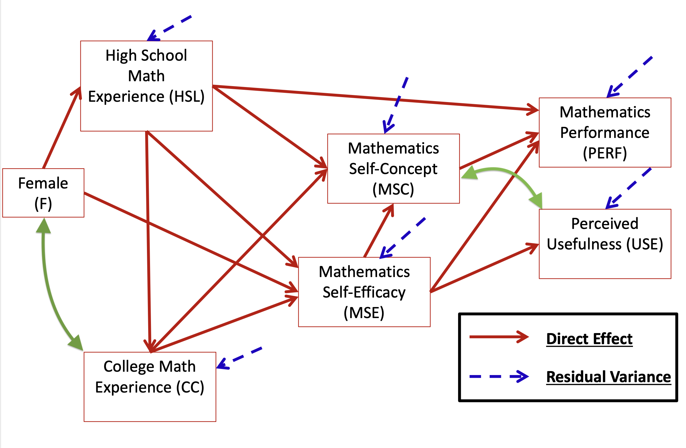{fig-align="center"}- The largest normalized covariances suggest relationships that may be present that are not being modeled: - Add a direct effect between F and CC - Add a direct effect between MSC and USE OR Add a residual covariance between MSC and USE## Model Midification Method 2: More Help for Fit- As we used Maximum Likelihood to estimate our model, another useful feature is that of the modification indices - Modification indices (also called Score or LaGrangian Multiplier tests) that attempt to suggest the change in the log-likelihood for adding a given model parameter (larger values indicate a better fit for adding the parameter)```{r}#calculate modification indicesmodel01.mi =modificationindices(model01.fit, sort. = T)#display values of indiceshead(model01.mi, 10)```- The modification indices have three large values: - A direct effect predicting MSC from USE - A direct effect predicting USE from MSC - A residual covariance between USE and MSC- Note: the MI value is -2 times the change in the log-likelihood and the EPC is the expected parameter value - The MI is like a 1 DF Chi-Square Deviance test - Values greater than 3.84 are likely to be significant changes in the log-likelihood- All three are for the same variable: so we can only choose one - This is where theory would help us decide- As we do not know theory, we will choose to add a residual covariance between USE and MSC ( the “\~\~” symbol) - Their covariance is unexplained by the model – not a great theoretical statement (but will allow us to make inferences if the model fits) - MI = 41.517 - EPC = 70.912# Model 2: New Model by adding MSE with USE## Model 2: `lavaan` syntax```{r}#model 02: Add residual covariance between USE and MSC-------------------------------------model02.syntax =" #endogenous variable equationsperf ~ hsl + msc + mseuse ~ msemse ~ hsl + cc + female msc ~ mse + cc + hslcc ~ hslhsl ~ female#endogenous variable interceptsperf ~ 1use ~ 1mse ~ 1msc ~ 1cc ~ 1hsl ~ 1#endogenous variable residual variancesperf ~~ perfuse ~~ usemse ~~ msemsc ~~ msccc ~~ cc hsl ~~ hsl#endogenous variable residual covariances#none specfied in the original model so these have zeros:perf ~~ 0*use + 0*mse + 0*msc + 0*cc + 0*hsluse ~~ 0*mse + msc + 0*cc + 0*hsl #<- the changed part of syntax here (no 0* in front of msc)mse ~~ 0*msc + 0*cc + 0*hslmsc ~~ 0*cc + 0*hslcc ~~ 0*hsl"```## Assessing Model fit of the Modified Model```{r}#estimate modelmodel02.fit =sem(model02.syntax, data=dataMath, mimic ="MPLUS", estimator ="MLR")summary(model02.fit, standardized =TRUE)#see if model convergedinspect(model02.fit, what="converged")``````{r}#| echo: true#| eval: false#show summary of model fit statistics and parameterssummary(model02.fit, standardized=TRUE, fit.measures=TRUE)``````{r}needed_fitIndex <-c("rmsea", "srmr","cfi", "tli", "chisq", "df", "pvalue") fitmeasures(model02.fit)[needed_fitIndex]```- Now we must start over with our path model decision tree - The model is identified (now 20 parameters \< 28 covariances) - Estimation converged; Standard errors look acceptable- Model fit indices: - The comparison with the saturated model suggests our model fits statistically - The RMSEA is 0.049, which indicates good fit - The CFI and TLI both indicate good fit (CFI/TLI \> .90) - The SRMR also indicates good fit- Therefore, we can conclude the model adequately approximates the covariance matrix – meaning we can now inspect our model parameters…but first, let’s check our residual covariances and modification indices## Normalized Residual Covariances```{r}residuals(model02.fit, type ="normalized")```- Only one normalized residual covariance is bigger than +/- 1.96: CC with Female - Given the number of covariances we have, this is likely okay## Modeification Indices for Model 2```{r}model02.mi =modificationindices(model02.fit, sort. = T)head(model02.mi, 10)```- Now, no modification indices are glaringly large, although some are bigger than 3.84 - We discard these as our model now fits (and adding them may not be meaningful)## More on Modification Indices- Recall from our original model that we received the following modification index values for the residual covariance between MSC and USE: - MI = 41.529 - EPC = 70.912```{r}model01.mi[2, ]```- The estimated residual covariance between MSC and USE in the modified model is: 70.249```{r}parameterestimates(model02.fit) |>filter(lhs =="use"& op =="~~"& rhs =="msc")```- The difference in log-likelihoods is: - -2\*(change) = 58.279```{r}anova(model01.fit, model02.fit)```- The values given by the MI and EPC are approximations## Model Parameter Investigation```{r}#| eval: falseRegressions: Estimate Std.Err z-value P(>|z|) Std.lv Std.all perf ~ hsl 0.1530.1071.4320.1520.1530.068 msc 0.0370.0094.1470.0000.0370.215 mse 0.1390.01310.7000.0000.1390.557 use ~ mse 0.2770.0733.8030.0000.2770.209 mse ~ hsl 4.1380.40610.2030.0004.1380.459 cc 0.3930.1053.7230.0000.3930.194 female 4.1681.1603.5930.0004.1680.166 msc ~ mse 0.7360.06611.1190.0000.7360.512 cc 0.5190.1174.4340.0000.5190.179 hsl 2.8240.5934.7640.0002.8240.218 cc ~ hsl 0.6620.2472.6860.0070.6620.149 hsl ~ female 0.2080.1541.3480.1780.2080.075```- There are two direct effects that are non-significant: - $\beta_{F, HSL} = .208$, p = .178 - $\beta_{HSL, PERF} = .153$, p = .152- We leave these in the model 2, but the overall path model seems to suggest they are not needed - So, I will remove them and re-estimate the model# Model 3: Remove non-significant effects## Model 3: `lavaan` syntax```{r}#| results: hide#model 03: removing HSL predicting PERF and Gender predicting HSL ----------------model03.syntax =" #endogenous variable equationsperf ~ msc + mseuse ~ msemse ~ hsl + cc + female msc ~ mse + cc + hslcc ~ hsl#endogenous variable interceptsperf ~ 1use ~ 1mse ~ 1msc ~ 1cc ~ 1#endogenous variable residual variancesperf ~~ perfuse ~~ usemse ~~ msemsc ~~ msccc ~~ cc #endogenous variable residual covariances#none specfied in the original model so these have zeros:perf ~~ 0*use + 0*mse + 0*msc + 0*cc use ~~ 0*mse + msc + 0*cc mse ~~ 0*msc + 0*cc msc ~~ 0*cc "#estimate modelmodel03.fit =sem(model03.syntax, data=dataMath, mimic ="MPLUS", estimator ="MLR")summary(model03.fit, fit.measures =TRUE)```## Model 3: Model fit results- We have: an identified model, a converged algorithm, and stable standard errors, so model fit should be inspected - Next – inspect model fit - Model fit seems to not be as good as we would think```{r}#see if model convergedinspect(model03.fit, what="converged")fitmeasures(model03.fit)[needed_fitIndex]```- Again, the largest normalized residual covariance is that of Female and CC```{r}residuals(model03.fit, type ="normalized")```- MI for direct effect of Female on CC is 5.090, indicating that adding this parameter may improve model fit```{r}modificationindices(model03.fit, sort. = T)[1:3,]```- So, we will now add a direct effect of Female on CC# Model 4: Adding Female on CC## Model 4: `lavaan` syntax```{r}#model 04: Add gender predicting cc -------------------------------------------------------------model04.syntax =" #endogenous variable equationsperf ~ msc + mseuse ~ msemse ~ (b_hsl_mse)*hsl + (b_cc_mse)*cc + female msc ~ mse + cc + hslcc ~ (b_hsl_cc)*hsl + female#endogenous variable interceptsperf ~ 1use ~ 1mse ~ 1msc ~ 1cc ~ 1#endogenous variable residual variancesperf ~~ perfuse ~~ usemse ~~ msemsc ~~ msccc ~~ cc #endogenous variable residual covariances#none specfied in the original model so these have zeros:perf ~~ 0*use + 0*mse + 0*msc + 0*cc use ~~ 0*mse + msc + 0*cc mse ~~ 0*msc + 0*cc msc ~~ 0*cc #indirect effect of interest:ind_hsl_mse := b_hsl_cc*b_cc_mse#total effect of interest:tot_hsl_mse := b_hsl_mse + (b_hsl_cc*b_cc_mse)"model04.fit =sem(model04.syntax, data=dataMath, mimic ="MPLUS", estimator ="MLR")```## Model 4: Model Fit Index```{r}inspect(model04.fit, what="converged")fitmeasures(model04.fit)[needed_fitIndex]residuals(model04.fit, type ="normalized")model04.mi <-modificationindices(model04.fit, sort. = T)head(model04.mi, 5)```- We have: an identified model, a converged algorithm, and stable standard errors, so model fit should be inspected- No normalized residual covariances are larger than +/- 1.96 – so we appear to have good fit- We will leave this model as-is and interpret the results## Model 4: Parameter Interpretation- Interpret each of these parameters as you would in regression: - A one-unit increase in HSL brings about a .695 unit increase in CC, holding Female constant - We can interpret the standardized parameter estimates for all variables except gender - A 1-SD increase in HSL means CC increases by 0.153 SD```{r}parameterestimates(model04.fit, standardized = T, ci = F) |>filter(op =="~")```## Model Interpretation: Explained Variability```{r}sort(inspect(model04.fit, what ='r2'))```- The R2 for each endogenous variable: - CC – 0.039 - USE – 0.041 - MSE – 0.298 - MSC – 0.485 - PERF – 0.576- Note how college experience and perceived usefulness both have low percentages of variance accounted for by the model - We could have increased the R2 for USE by adding the direct path between MSC and USE instead of the residual covariance## Overall Model Interpretation- High School Experience and Female are significant predictors of College Experience ($\beta_{HSL, CC} = .695, p = .006$ and $\beta_{F, CC} = -1.662, p = .021$) - Females lower than males in College Experience - More High School Experience means more College Experience- High School Experience, College Experience, and Gender are significant predictors of Math Self-Efficacy ($\beta_{HSL, MSE}= 4.05, p < .001$; $\beta_{CC, MSE}= .383, p < .001$; $\beta_{F, MSE}= 3.819, p = .001$) - More High School and College Experience means higher Math Self-Efficacy - Females have higher Math Self-Efficacy than Men- High School Experience, College Experience, and Math Self-Efficacy are significant predictors of Math Self-Concept ($\beta_{HSL, MSC}= 2.894, p < .001$; $\beta_{CC, MSC}= .545, p < .001$; $\beta_{MSE, MSC}= .692, p < .001$) - More High School and College Experience and higher Math Self-Efficacy mean higher Math Self-Concept- Higher Math Self-Efficacy means significantly higher Perceived Usefulness- Higher Math Self-Efficacy and Math Self-Concept result in higher Math Performance scores- Math Self-Concept and Perceived Usefulness have a significant residual covariance## Wrapping Up- In this lecture we discussed the basics of path analysis - Model specification/identification - Model estimation - Model fit (necessary, but not sufficient) - Model modification and re-estimation - Final model parameter interpretation- There is a lot to the analysis – but what is important to remember is the over-arching principal of multivariate analyses: covariance between variables is important - Path models imply very specific covariance structures - The validity of the results hinge upon accurately finding an approximation to the covariance matrix### Next Class1. Indirect effect2. Causality3. Hypothesis tests4. Robust ML