---
title: "Lecture 09"
subtitle: "Generalized Measurement Models: Modeling Observed Dichotomous Data"
author: "Jihong Zhang"
institute: "Educational Statistics and Research Methods"
title-slide-attributes:
data-background-image: ../Images/title_image.png
data-background-size: contain
execute:
echo: true
eval: false
warning: false
format:
html:
code-tools: true
code-line-numbers: false
code-fold: true
code-summary: 'Click here to see R code'
number-offset: 1
fig.width: 10
fig-align: center
message: false
revealjs:
output-file: slides-index.html
logo: ../Images/UA_Logo_Horizontal.png
incremental: false # choose "false "if want to show all together
transition: slide
background-transition: fade
theme: [simple, ../pp.scss]
footer: <https://jihongzhang.org/posts/2024-01-12-syllabus-adv-multivariate-esrm-6553>
scrollable: true
slide-number: true
chalkboard: true
number-sections: false
code-line-numbers: true
code-annotations: below
code-copy: true
code-summary: ''
highlight-style: arrow
view: 'scroll' # Activate the scroll view
scrollProgress: true # Force the scrollbar to remain visible
mermaid:
theme: neutral
#bibliography: references.bib
---
## Previous Class
1. Dive deep into factor scoring
2. Show how different initial values affect Bayesian model estimation
3. Show how parameterization differs for standardized latent variables vs. marker item scale identification
## Today's Lecture Objectives
1. Show how to estimate unidimensional latent variable models with dichotomous data
1. Also know as [Item response theory]{.underline} (IRT) or [Item factor analysis]{.underline} (IFA)
2. Show how to estimate different parameterizations of IRT/IFA models
3. Describe how to obtain IRT/IFA auxiliary statistics from Markov Chains
4. Show variations of various dichotomous-data models.
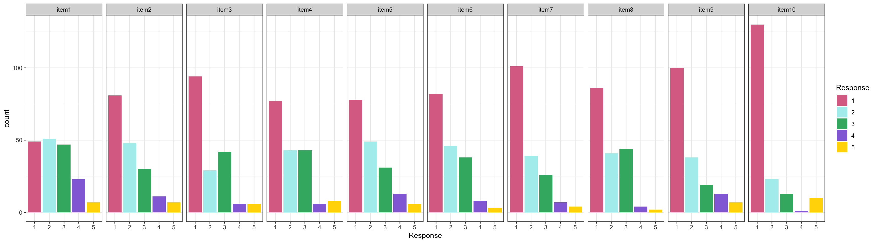
## Example Data: Conspiracy Theories
- Today's example is from a bootstrap resample of 177 undergraduate students at a large state university in the Midwest.
- The survey was a measure of 10 questions about their beliefs in various conspiracy theories that were being passed around the internet in the early 2010s
- All item responses were on a 5-point Likert scale with:
1. Strong Disagree $\rightarrow$ 0
2. Disagree $\rightarrow$ 0
3. Neither Agree nor Disagree $\rightarrow$ 0
4. Agree $\rightarrow$ 1
5. Strongly Agree $\rightarrow$ 1
- The purpose of this survey was to study individual beliefs regarding conspiracies.
- Our purpose in using this instrument is to provide a context that we all may find relevant as many of these conspiracies are still prevalent.
## Make Our Data Dichotomous ([not a good idea in practice]{.underline})
To show dichotomous-data models with our data, we will arbitrarilly dichotomize our item responses:
- {0}: Response is *Strongly disagree or disagree, or Neither* (1-3)
- {1}: Response is *Agree, or Strongly agree* (4-5)
Now, we could argue that a **1** represents someone who agrees with a statement and **0** represents someone who disagrees or is neutral.
Note that this is only for illustrative purpose, such dichotomization shouldn't be done because
- There are distributions for multinomial categories
- The results will reflect more of our choice for 0/1
But we first learn dichotomous data models before we get to models for polytomous models.
## Examining Dichotomous Data
```{r}
#| fig-width: 18
#| eval: true
library(tidyverse)
library(kableExtra)
library(here)
library(blavaan)
self_color <- c("#DB7093", "#AFEEEE", "#3CB371", "#9370DB", "#FFD700")
root_dir <- "teaching/2024-01-12-syllabus-adv-multivariate-esrm-6553/Lecture07/Code"
dat <- read.csv(here(root_dir, 'conspiracies.csv'))
itemResp <- dat[,1:10]
colnames(itemResp) <- paste0('item', 1:10)
conspiracyItems = itemResp
itemResp |>
  rownames_to_column("ID") |>
  pivot_longer(-ID, names_to = "Item", values_to = "Response") |>
  mutate(Item = factor(Item, levels = paste0('item', 1:10)),
         Response = factor(Response, levels = 1:5)) |>
  ggplot() +
  geom_bar(aes(x = Response, fill = Response, group = Response),
           position = position_stack()) +
  facet_wrap(~ Item, nrow = 1, ncol = 10) +
  theme_bw() +
  scale_fill_manual(values = self_color)
conspiracyItemsDichtomous <- itemResp |>
  mutate(across(everything(), \(x) ifelse(x <= 3, 0, 1)))
```
::: callout-note
## Note
These items have a relatively low proportion of people agreeing with each conspiracy statement
- Highest mean: .69
- Lowest mean: .034
:::
## Dichotomous Data Distribution: Bernoulli
The Bernoulli distribution is a one-trial version of the Binomial distribution
- Sample space (support) $Y \in {0,1}$
The probability mass function:
$$
P(Y=y)=\pi^y(1-\pi)^{1-y}
$$
The Bernoulli distribution has only one parameter: $\pi$ (typically, known as the probability of success: Y=1)
- Mean of the distribution: $E(Y)=\pi$
- Variance of the distribution: $Var(Y)=\pi(1-\pi)$
## Definition: Dichotomous vs. Binary
Note the definitions of some of the words for data with two values:
- Dichotomous: Taking two values (without numbers attached)
- Binary: either zero or one
Therefore:
1. Not all dichotomous variable are binary, i.e., {2,7} is a dichotomous but not binary variable
2. All binary variables are dichotomous
Finally:
1. Bernoulli distributions are for binary variables
2. Most dichotomous variables can be recorded as binary variables without loss of model effects
## Models with Bernoulli Distributions
Generalized linear models using Bernoulli distributions put a linear model onto a transformation of the mean
- [Link function]{.underline} maps the mean $E(Y)$ from its original range of \[0,1\] to (-$\infty$, $\infty$);
- For an unconditional (empty) model, this is shown here:
$$
f(E(Y)) =f(\pi)
$$
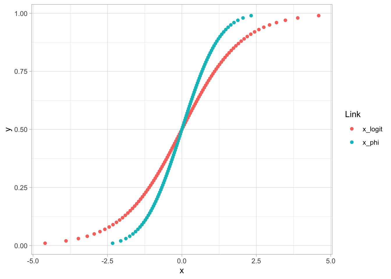
## Link Functions for Bernoulli Distributions
Common choices for the link function in [latent variable modeling]{.underline}:
1. Logit (or log odds):
$$
f(\pi)=\log(\frac\pi{1-\pi})
$$
2. Probit:
$$
f(\pi)=\Phi^{-1}(\pi)
$$
Where $\Phi$ is the inverse cumulative distribution of a standard normal distribution
$$
\boldsymbol{\Phi}(Z)=\int_{-\infty}^Z\frac1{\sqrt{2\pi}}\exp(\frac{-x^2}{2})dx
$$
------------------------------------------------------------------------
### Visualization of Logit and Probit
```{r}
#| eval: true
#| echo: true
tibble(
  y = seq(.01, .99, .01),
  x_logit = log(y / (1 - y)),
  x_phi = qnorm(y)
  ) |>
  pivot_longer(starts_with('x_'), names_to = 'Link', values_to = "x") |>
  ggplot() +
  geom_point(aes(x, y, col = Link)) +
  theme_light()
```
------------------------------------------------------------------------
## Less Common Link Functions
In the generalized linear models literature, there are a number of different link functions:
- Log-log: $f(\pi)=-\log(-\log(\pi))$
- Complementary Log-log: $f(\pi)=\log(-\log(1-\pi))$
Most of these seldom appear in latent variable models
- Each has a slightly different curve shape
## Inverse Link Functions
Our latent variable models will be defined on the scale of the link function
- Sometimes we wish to convert back to the scale of the data
- Example: **Test characteristic curves** mapping $\theta_p$ onto an expected test score
For this, we need the inverse link function
- Logit (or log odds) link function:
$$
\text{logit}(\pi)=\log(\frac\pi{1-\pi})
$$
- Logit (or log odds) inverse link function:
$$
\pi=\frac{\exp(logit(\pi))}{1+\exp(logit(\pi))} \\
= \frac1{1+\exp(-logit(\pi))} \\
= (1 + \exp(-logit(\pi)))^{-1}
$$
# Latent Variable Models with Bernoulli Distributions
## Define Latent Variable Models with Bernoulli Distributions
To define a LVM for binary responses using a Bernoulli Distribution
- To start, we will use the logit link function
- We will begin with the linear predictor we had from the normal distribution models ([*Confirmatory factor analysis*]{.underline}: $\mu_i + \lambda_i\theta_p)$
For an item $i$ and a person $p$, the model becomes:
$$
P(Y_{pi}=1|\theta_p) = \text{logit}^{-1}(\mu_i + \lambda_i\theta_p)
$$
- Note: the mean $\pi_i$ is replaced by $P(Y_{pi}=1|\theta_p)$
- This is the mean of the observed variable, conditional on $\theta_p$;
- The item intercept (easiness, location) is $\mu_i$: the expected logit when $\theta_p=0$
- The item discrimination is $\lambda_i$: the change in the logit for a one-unit increase in $\theta_p$
## Extension: A more general form
A 3-PL Item Response Theory Model with same statistical form but different notations:
$$
P(Y_{pi}=1|\theta_p,c_i,a_i,b_j)=c_i+(1-c_i)\text{logit}^{-1}(\alpha_i\theta_p+d_i)
$$
$$
P(Y_{pi}=1|\theta_p,c_i,a_i,b_j)=c_i+(1-c_i)\text{logit}^{-1}(\alpha_i(\theta_p-b_i))
$$
where
- $\theta_p$ is the latent variable for examinee $p$, representing the examinee's proficiency such that higher values indicate more proficency
- $a_i$, $d_i$, $c_i$ are item parameters:
- $a_i$: the capability of item to discriminate between examinees with lower and higher values along the latent variables;
- $d_i$: item "easiness"
- $b_i$: item "difficulty", $b_i=d_i/(-a_i)$
- $c_i$: "pseudo-guessing" parameter – examinees with low proficiency may have a nonzero probability of a correct response due to guessing
## Model Family Names
Depending on your field, the model from the previous slide can be called:
- The two-parameter logistic (2PL) model with slope/intercept parameterization
- An item factor model
These names reflect the terms given to the model in diverging literature:
- 2PL: Education measurement
> Birnbaum, A. (1968). Some Latent Trait Models and Their Use in Inferring an Examinee’s Ability. In F. M. Lord & M. R. Novick (Eds.), Statistical Theories of Mental Test Scores (pp. 397-424). Reading, MA: Addison-Wesley.
- Item factor analysis: Psychology
> Christofferson, A.(1975). Factor analysis of dichotomous variables. Psychometrika , 40, 5-22.
Estimation methods are the largest difference between the two families.
## Differences from Normal Distributions
Recall our [normal distribution models]{.underline}:
$$
Y_{pi}=\mu_i+\lambda_i\theta_p+e_{p,i};\\
e_{p,i}\sim N(0, \psi_i^2)
$$
Compared to our [Bernoulli distribution models]{.underline}:
$$
logit(P(Y_{pi}=1))=\mu_i+\lambda_i\theta_p
$$
Differences:
1. No residual (unique) variance components $\psi_i^2$ in Bernoulli distribution;
2. Only one parameter in the distribution; variance is a function of the mean;
3. Identity link function in normal distribution: $f(E(Y_{pi}|\theta_p))=E(Y_{pi}|\theta_p)$
- Model scale and data scale are the same
4. Logit link function in Bernoulli distribution
- Model scale is different from data scale
## From Model Scale to Data Scale
Commonly, the IRT or IFA model is shown on the data scale (using the inverse link function):
$$
P(Y_{pi}=1)=\frac{\exp(\mu_i+\lambda_i\theta_p)}{1+\exp(\mu_i+\lambda_i\theta_p)}
$$
The core of the model (the terms in the exponent on the right-hand side) is the same
Models are equivalent:
1. $P(Y_{pi}=1)$ is on the data scale;
2. $logit(P(Y_{pi}=1))$ is on the model (link) scale;
## Modeling All Data
As with the normal distribution (CFA) models, we use the Bernoulli distribution for all observed variables:
$$
logit(P(Y_{p1}=1))=\mu_1+\lambda_1\theta_p \\
logit(P(Y_{p2}=1))=\mu_2+\lambda_2\theta_p \\
logit(P(Y_{p3}=1))=\mu_3+\lambda_3\theta_p \\
logit(P(Y_{p4}=1))=\mu_4+\lambda_4\theta_p \\
logit(P(Y_{p5}=1))=\mu_5+\lambda_5\theta_p \\
\dots \\
logit(P(Y_{p10}=1))=\mu_{10}+\lambda_{10}\theta_p \\
$$
## Measurement Model Analysis Procedure
1. Specify model
2. Specify scale identification method for latent analysis
3. Estimate model
4. Examine model-data fit
5. Iterate between steps 1-4 until adequate fit is achieved
**Measurement Model Auxiliary Steps:**
1. Score estimation (and secondary analysis with scores)
2. Item evaluation
3. Scale construction
4. Equating
5. Measurement invariance / differential item functioning
## Model Specification
The set of equations on the previous slide formed [**Step #1**]{.underline} of the Measurement Model Analysis
1. Specify Model
The next step is:
2. Specify scale identification method for latent variables
We will initially assume $\theta_p \sim N(0,1)$, which allows us to estimate all item parameters of the model, that we call standardization
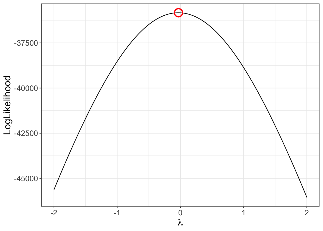
## Likelihood Functions
The likelihood of [**item 1**]{.underline} is the function of production of all individuals' responses:
$$
f(Y_{pi}|\lambda_1)=\prod_{p=1}^{P}(\pi_{p1})^{Y_{p1}}(1-\pi_{p1})^{1-Y_{p1}}
$$ {#eq-likelihood}
To simplify @eq-likelihood, we take the log:
$$
\log f(Y_{pi}|\lambda_1)=\Sigma_{p-1}^{P}\log[(\pi_{p1})^{Y_{pi}}(1-\pi_{p1})^{1-Y_{pi}}]
$$ {#eq-loglikelihood}
Since we know from logit function that:
$$
\pi_{pi}=\frac{\exp(\mu_1+\lambda_1\theta_p)}{1+\exp(\mu_1+\lambda_1\theta_p)}
$$
Which then becomes:
$$
\log f(Y_{pi}|\lambda_1)=\Sigma_{p-1}^{P}\log[(\frac{\exp(\mu_1+\lambda_1\theta_p)}{1+\exp(\mu_1+\lambda_1\theta_p)})^{Y_{pi}}(1-\frac{\exp(\mu_1+\lambda_1\theta_p)}{1+\exp(\mu_1+\lambda_1\theta_p)})^{1-Y_{pi}}]
$$
## Model (Data) Log Likelihood Functions
As an example for $\lambda_1$:
```{r}
#| eval: true
lambdas = seq(-2, 2, .01)
mu1 = 1
thetas = rnorm(nrow(conspiracyItemsDichtomous))
Y = conspiracyItemsDichtomous[,1]
```
```{r}
#| eval: true
#| cache: true
#| echo: true
LogLike <- function(lambda){
  ll = sapply(1:length(Y), \(x){
   log((exp(mu1+thetas*lambda)/(1+exp(mu1+thetas*lambda)))^Y[x]*(1-(exp(mu1+thetas*lambda)/(1+exp(mu1+thetas*lambda))))^(1-Y[x]))
  })
  sum(ll)
}
LogLike_dat <- tibble(
  x = lambdas,
  y = sapply(lambdas, LogLike)
)
LogLike_dat |>
  ggplot() +
  geom_line(aes(x, y)) +
  annotate("point", x = lambdas[which.max(LogLike_dat$y)], y = max(LogLike_dat$y),
             col = "red", size = 5, shape = 1, stroke = 1.4) +
  labs(x = expression(lambda), y = 'LogLikelihood') +
  theme_bw() +
  theme(text = element_text(size = 15))
```
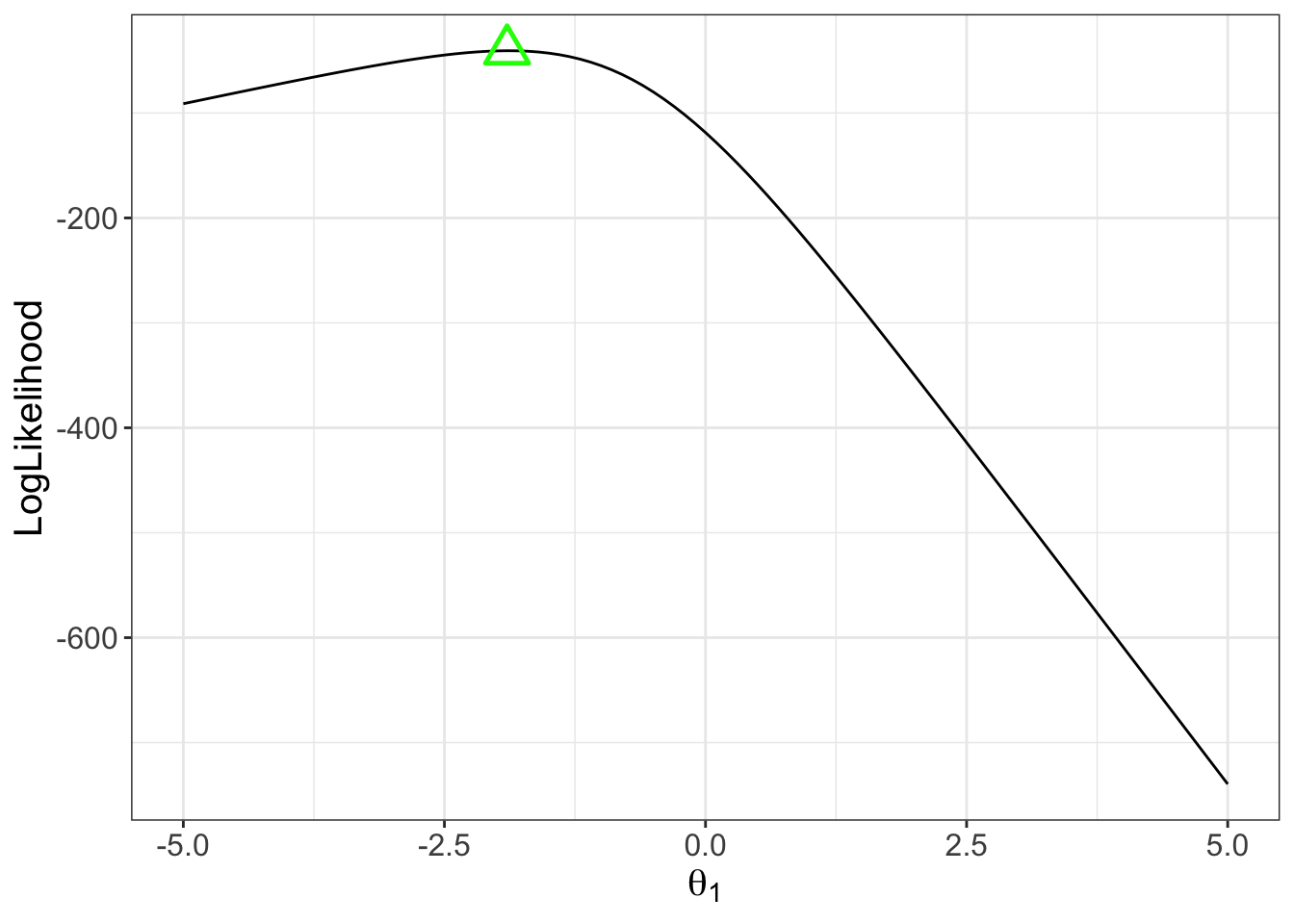
## Model (Data) Log Likelihood Function for $\theta$
For each person, the same model likelihood function is used
- Only now it varies across each item response
- Example: Person 1
$$
f(Y_{1i}|\theta_1)=\prod_{i=1}^{I}(\pi_{1i})^{Y_{1i}}(1-\pi_{1i})^{1-Y_{1i}}
$$
```{r}
#| eval: true
#| cache: true
#| echo: true
#| warning: false
LogLike2 <- function(theta, lambda){
  mu1 = 1
  ll = sapply(1:length(seq(-5, 5, .1)), \(x){
   log((exp(mu1+theta*lambda)/(1+exp(mu1+theta*lambda)))^Y[x]*
         (1-(exp(mu1+theta*lambda)/(1+exp(mu1+theta*lambda))))^(1-Y[x]))
  })
  sum(ll)
}

LogLike_dat2 <- tibble(
  x = seq(-5, 5, .1),
  y = sapply(seq(-5, 5, .1),
             \(x) LogLike2(x, lambda = 1.5))
)
LogLike_dat2 |>
  ggplot() +
  geom_line(aes(x, y)) +
  annotate("point", x = seq(-5, 5, .1)[which.max(LogLike_dat2$y)],
           y = max(LogLike_dat2$y),
           col = "green", size = 5, shape = 2, stroke = 1.3) +
  labs(x = expression(theta[1]), y = 'LogLikelihood') +
  theme_bw() +
  theme(text = element_text(size = 15))
```
# Implementing Bernoulli Outcomes in Stan
## Stan's `model` Block
```{stan, output.var='display'}
#| echo: true
model {

  lambda ~ multi_normal(meanLambda, covLambda); // Prior for item discrimination/factor loadings
  mu ~ multi_normal(meanMu, covMu);             // Prior for item intercepts

  theta ~ normal(0, 1);                         // Prior for latent variable (with mean/sd specified)

  for (item in 1:nItems){
    Y[item] ~ bernoulli_logit(mu[item] + lambda[item]*theta);
  }

}
```
For logit models without lower / upper asymptote parameters, `Stan` has a convenient `bernoulli_logit` function
- Automatically has the link function embedded
- The catch: The data has to be defined as an integer
Also, note that there are few differences from the model with normal outcomes (CFA)
- No $\psi$ parameters
## Stan's `parameters` Block
```{stan, output.var='display'}
#| echo: true
parameters {
  vector[nObs] theta;                // the latent variables (one for each person)
  vector[nItems] mu;                 // the item intercepts (one for each item)
  vector[nItems] lambda;             // the factor loadings/item discriminations (one for each item)
}
```
Only change from normal outcomes (CFA) model:
- No $\psi$ (psi) parameters
## Stan's `data{}` Block
```{stan, output.var='display'}
#| echo: true
data {
  int<lower=0> nObs;                            // number of observations
  int<lower=0> nItems;                          // number of items
  array[nItems, nObs] int<lower=0, upper=1>  Y; // item responses in an array

  vector[nItems] meanMu;             // prior mean vector for intercept parameters
  matrix[nItems, nItems] covMu;      // prior covariance matrix for intercept parameters

  vector[nItems] meanLambda;         // prior mean vector for discrimination parameters
  matrix[nItems, nItems] covLambda;  // prior covariance matrix for discrimination parameters
}
```
One difference from normal outcome model:
`array[nItems, nObs] int<lower=0, upper=1> Y;`
- Arrays are types of matrices (with more than two dimensions possible)
- Allows for different types of data (here Y are integers)
- Integer-valued variables needed for `bernoulli_logit()` function
- Arrays are row-major (meaning order of items and persons is switched)
- Can define differently
## Change to Data List for Stan Import
The switch of items and observations in the `array` statement means the data imported have to be transposed:
```{r}
#| eval: false
#| echo: true
modelIRT_2PL_SI_data = list(
  nObs = nObs,
  nItems = nItems,
  Y = t(conspiracyItemsDichtomous),
  meanMu = muMeanVecHP,
  covMu = muCovarianceMatrixHP,
  meanLambda = lambdaMeanVecHP,
  covLambda = lambdaCovarianceMatrixHP
)
```
## Running the Model in `Stan`
The `Stan` program takes longer to run than in linear models:
- Number of parameters: 197
- 10 observed variables: $\mu_i$ and $\lambda_i$ for $i = 1\dots10$
- 177 latent variables: $\theta_p$ for $p=1\dots177$
- `cmdstanr` samples call:
```{r}
#| eval: false
#| echo: fenced
modelIRT_2PL_SI_samples = modelIRT_2PL_SI_stan$sample(
data = modelIRT_2PL_SI_data,
seed = 02112022,
chains = 4,
parallel_chains = 4,
iter_warmup = 5000,
iter_sampling = 5000,
init = function() list(lambda=rnorm(nItems, mean=5, sd=1))
)
```
- Note: typically, longer chains are needed for larger models like this
- Note: Starting values added (mean of 5 is due to logit function limits)
- Helps keep definition of parameters (stay away from opposite mode)
- Too large of value can lead to `NaN` values (exceeding numerical precision)
## Model Results
```{r}
#| eval: true
library(cmdstanr)
save_dir <- "~/Library/CloudStorage/OneDrive-Personal/2024_Spring/ESRM6553 - Advanced Multivariate Modeling/Lecture09/"
modelIRT_2PL_SI_samples <- readRDS(here(save_dir, "modelIRT_2PL_SI_samples.RDS"))
```
Check convergence with $\hat R$ (PSRF):
```{r}
#| eval: true
summary(modelIRT_2PL_SI_samples$summary(.cores =4)['rhat'])
```
- Item Parameter Results:
```{r}
#| eval: true
modelIRT_2PL_SI_samples$summary(c('mu', 'lambda'), .cores =4)
```
## Modeling Strategy vs. Didactic Strategy
At this point, one should investigate model fit of the model we just ran (PPP, WAIC, LOO)
- If the model does not fit, then all model parameters could be biased
- Both item parameters and person parameters ($\mu_i$, $\lambda_i$, $\theta_p$)
- Moreover, the uncertainty accompanying each parameter (the posterior standard deviation) may also be biased
- Especially bad for psychometric models as we quantify reliability with these numbers
## Investigating Item Parameters
One plot that can help provide information about the item parameters is the item characteristic curve (ICC)
- The ICC is the plot of the expected value of the response conditional on the value of the latent traits, for a range of latent trait values
$$
E(Y_{pi}|\theta_p)=\frac{\exp(\mu_i+\lambda_i\theta_p)}{1+\exp(\mu_i+\lambda_i\theta_p)}
$$
- Because we have sampled values for each parameter, we can plot one ICC for each posterior draws
## Posterior ICC Plots
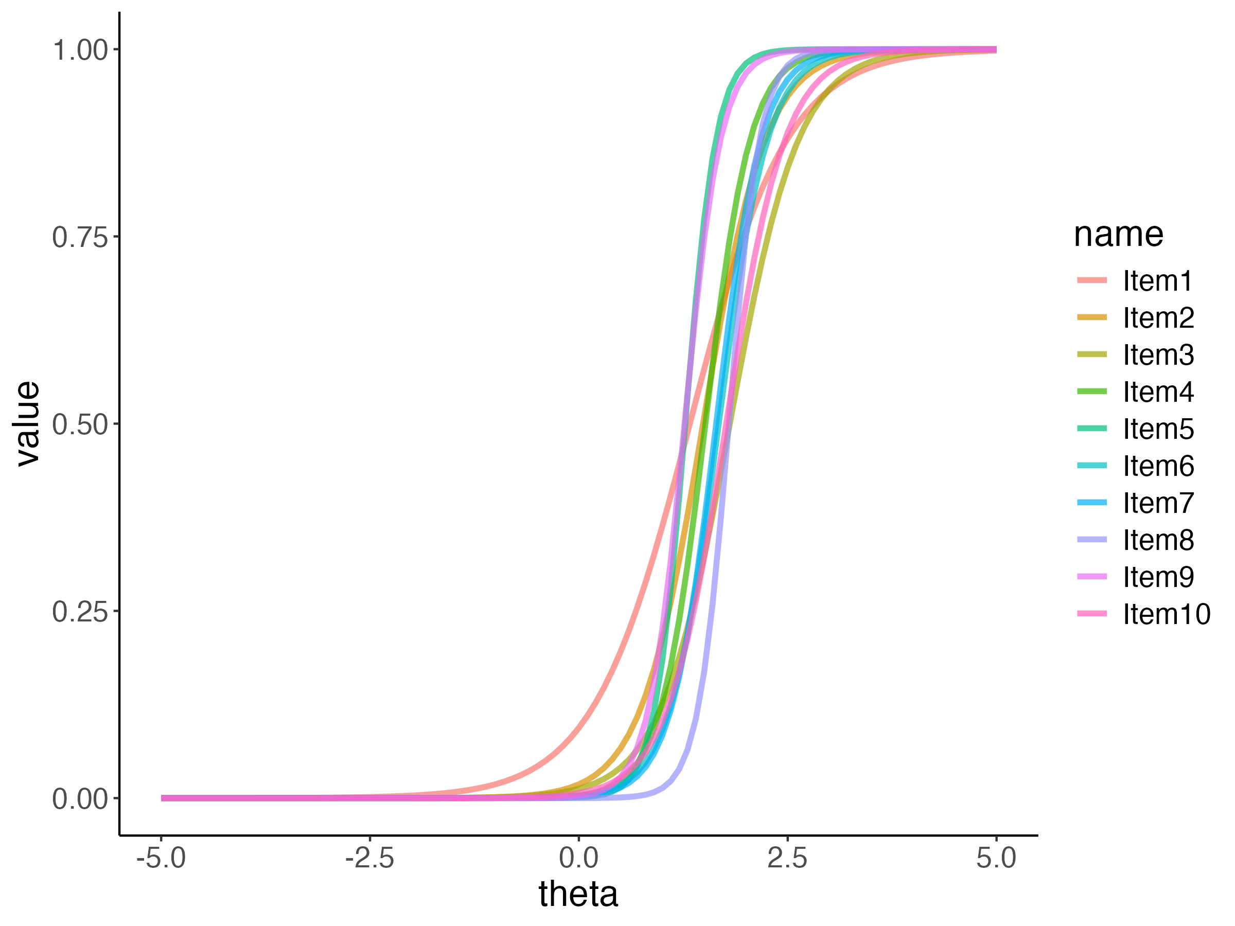{fig-align="center"}
## Item 5 ICC
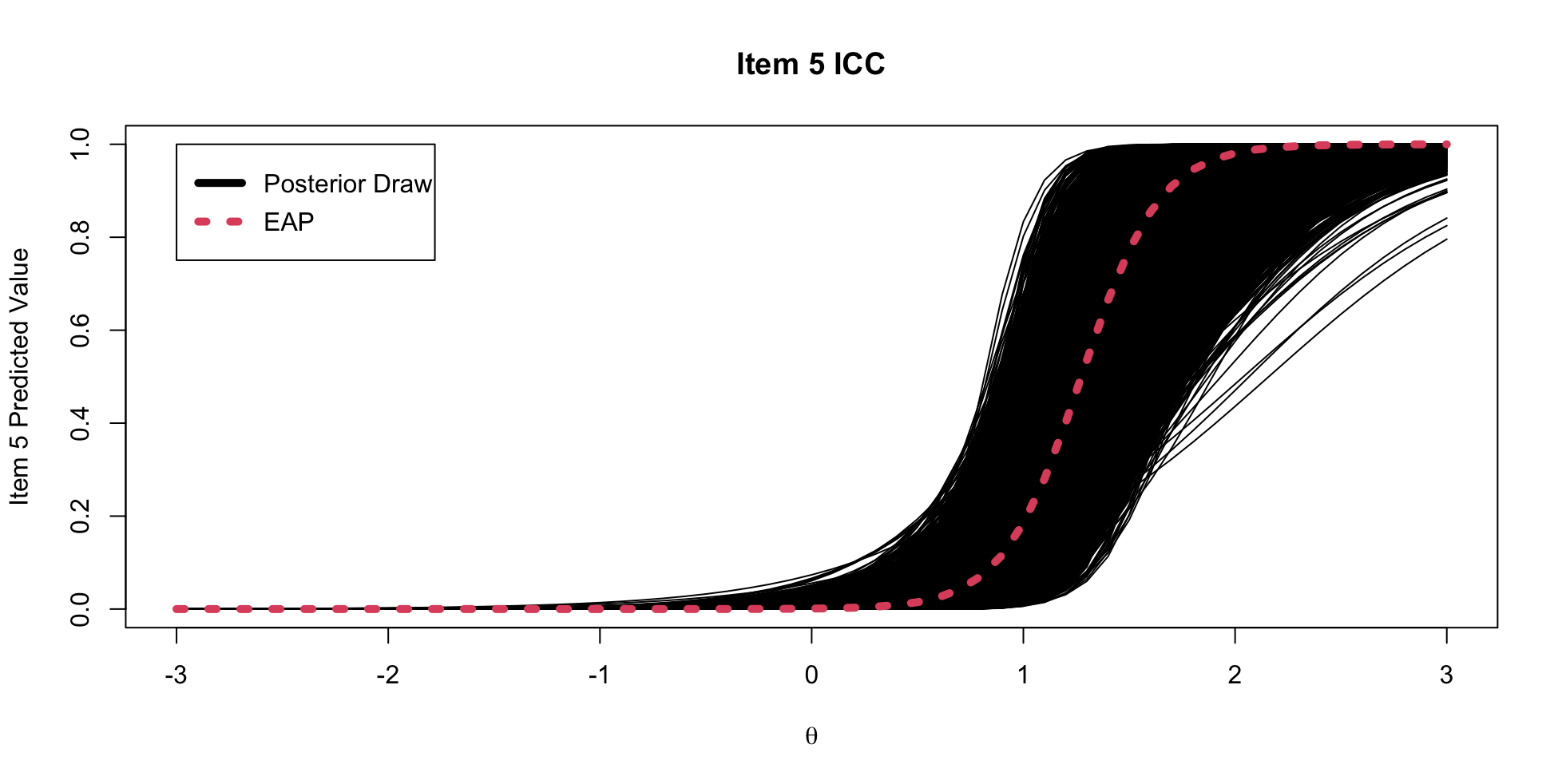{fig-align="center"}
# Investigating the Item Parameters
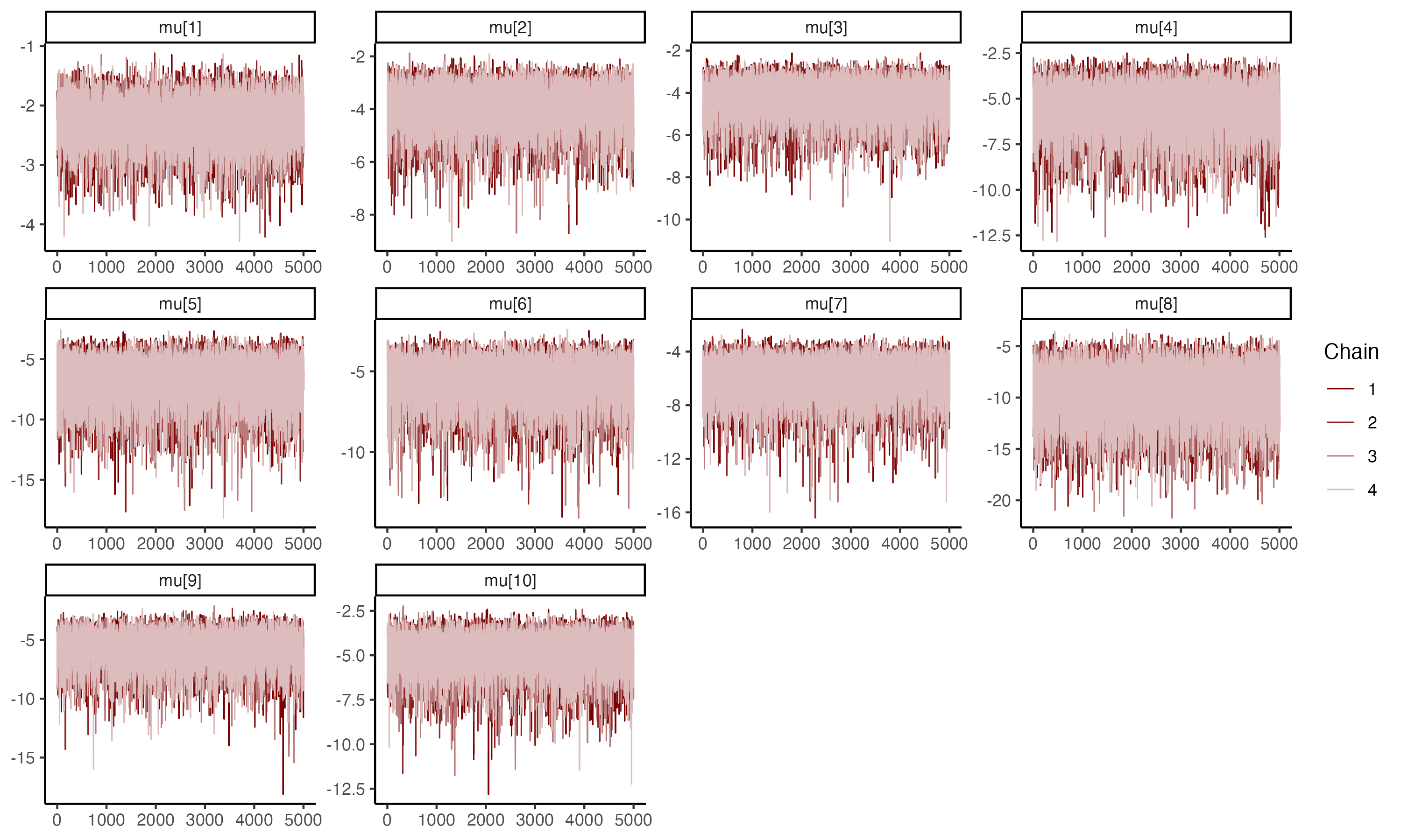
## Trace plots for $\mu_i$
{fig-align="center"}
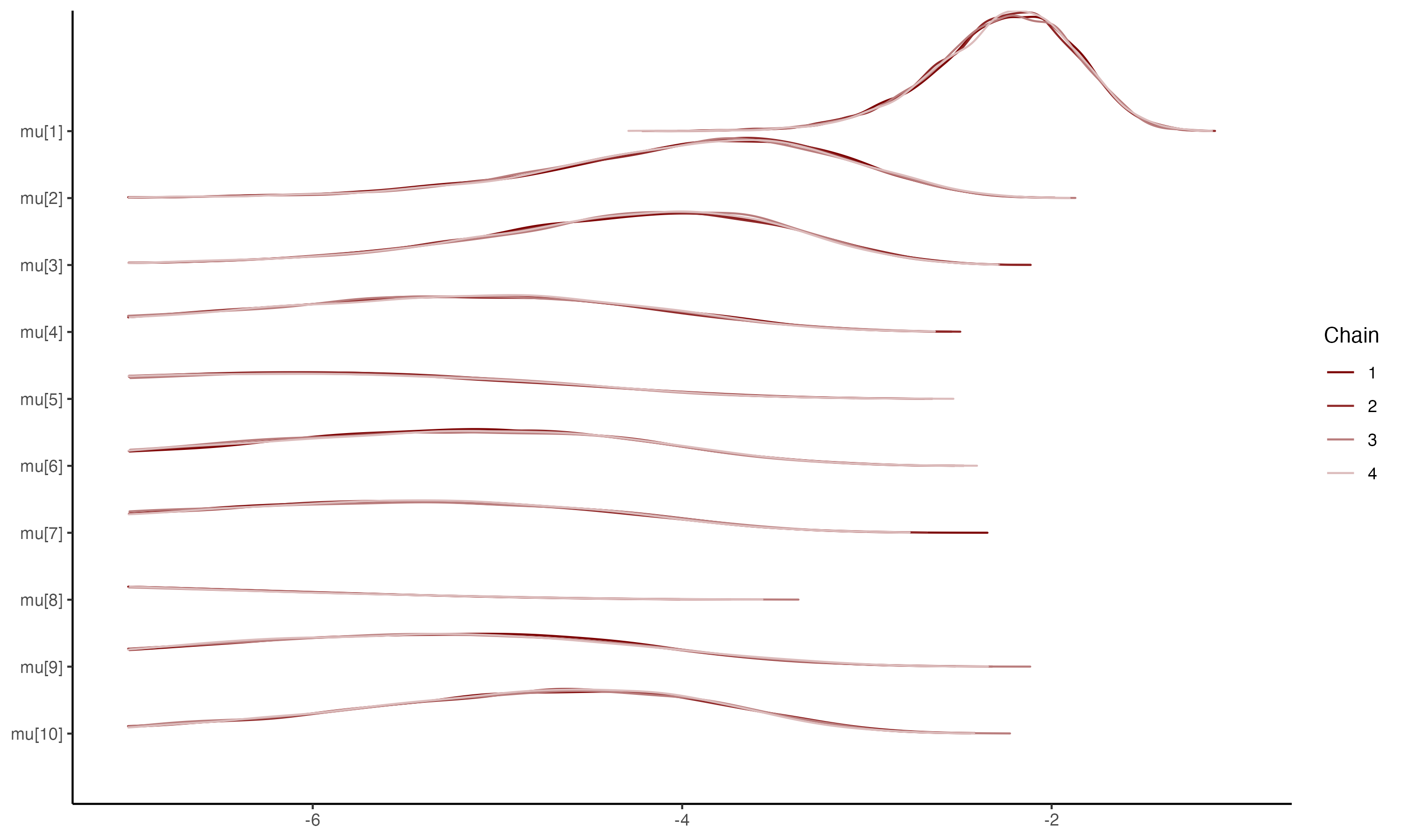
## Density plots for $\mu_i$
{fig-align="center"}
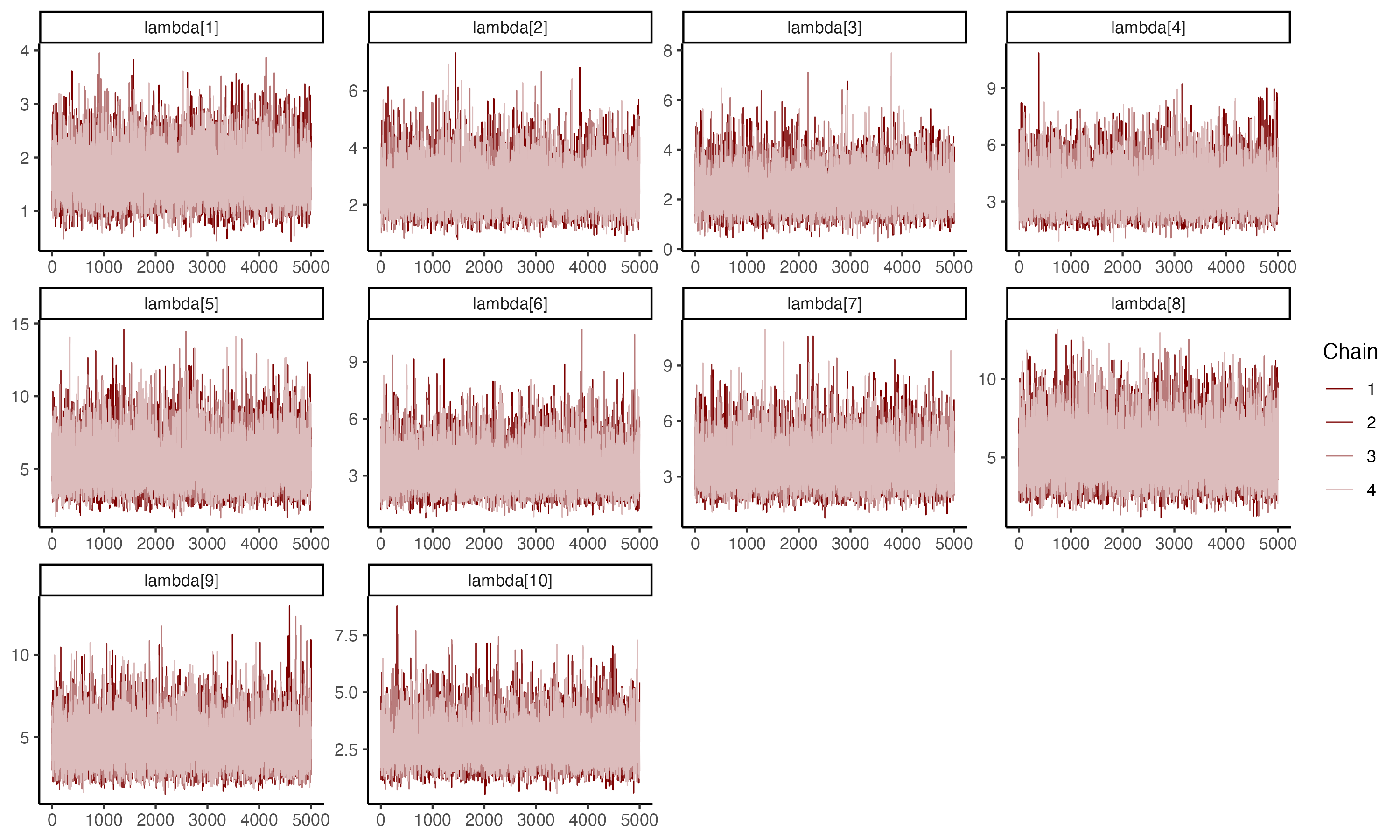
## Trace plots for $\lambda_i$
## 
## Density plots for $\lambda_i$
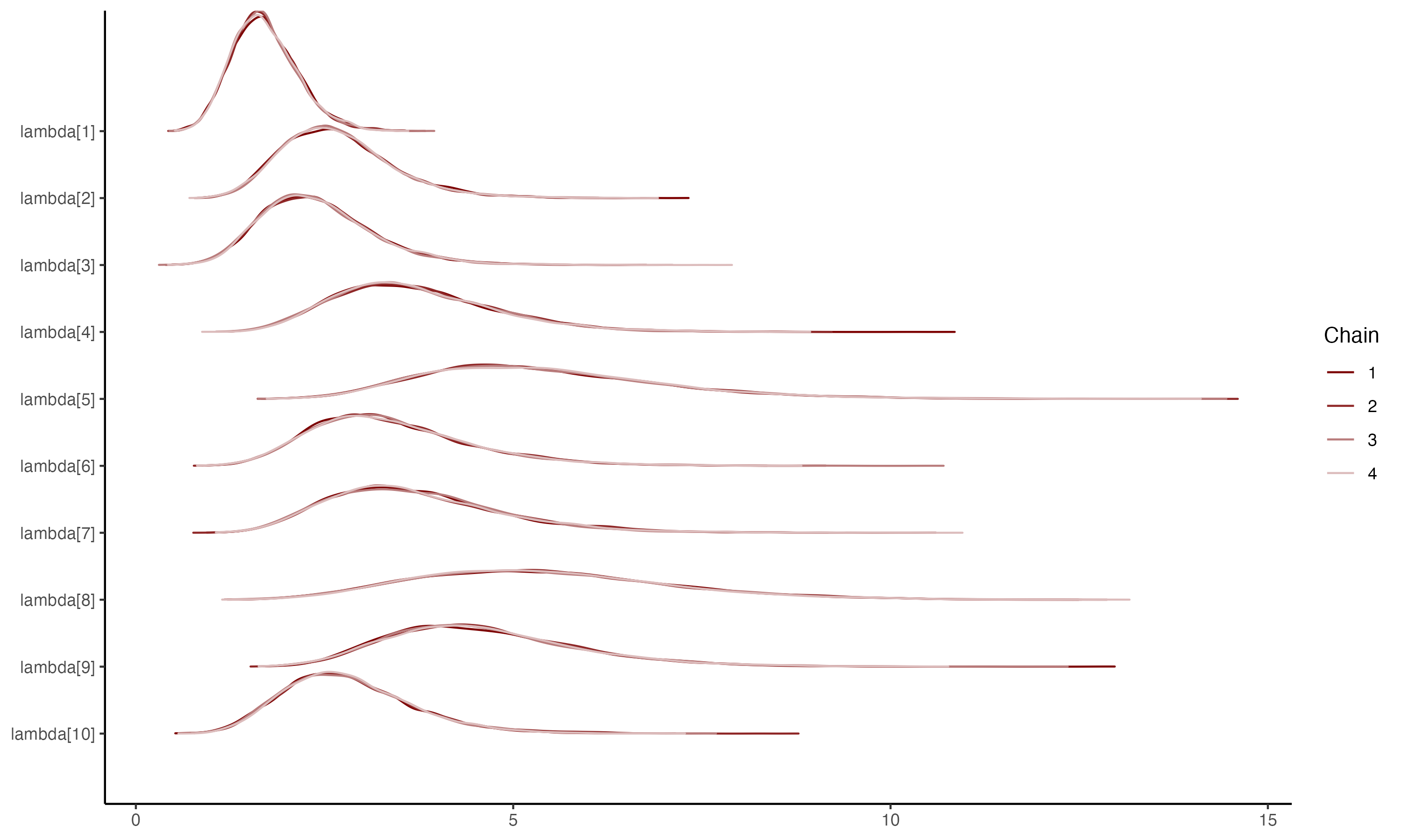{fig-align="center"}
## Bivariate plots for $\mu_i$ and $\lambda_i$
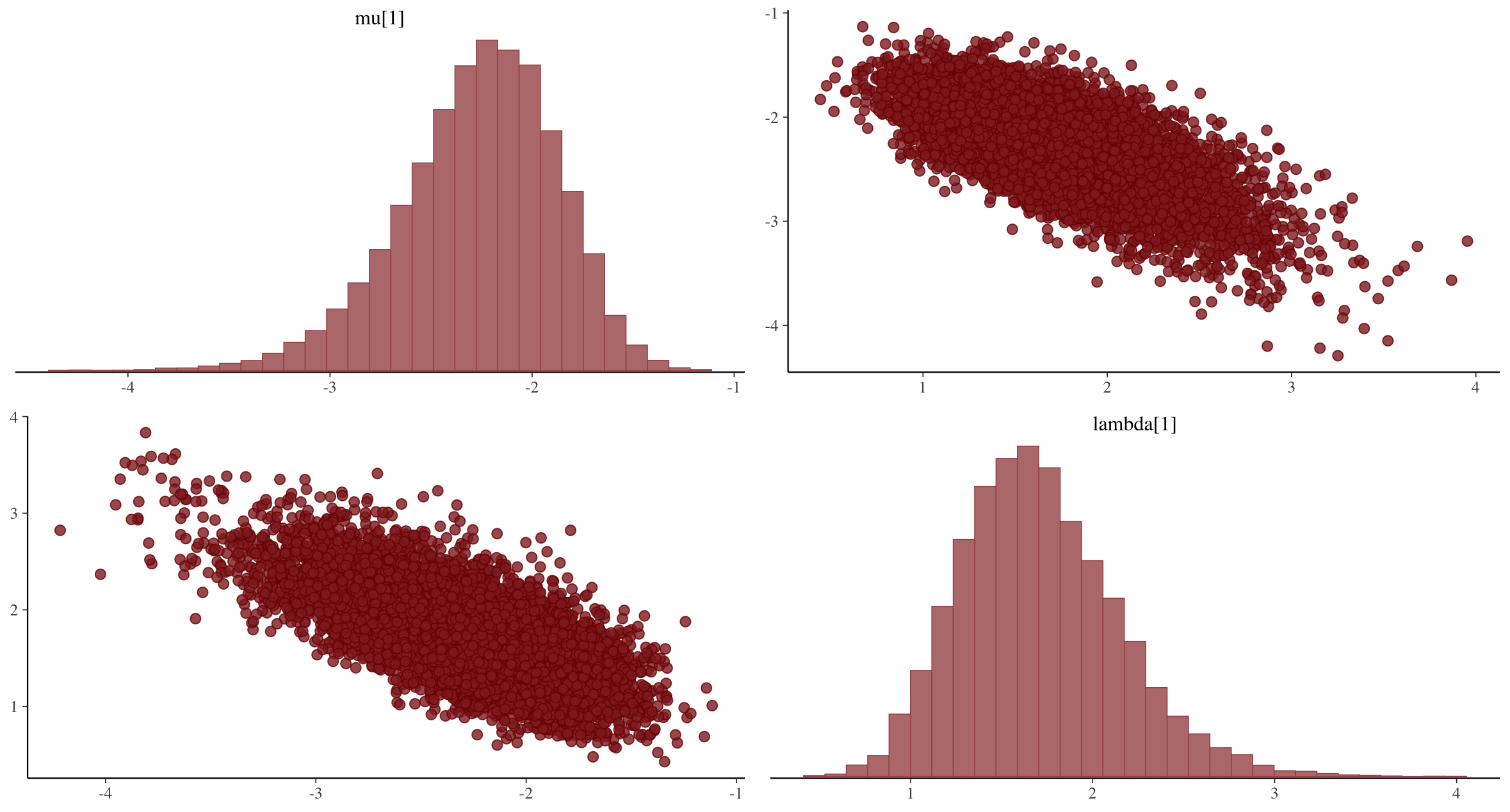{fig-align="center"}
## Latent Variables
```{r}
#| eval: true
print(modelIRT_2PL_SI_samples$summary(variables = "theta", .cores='4'), n=Inf)
```
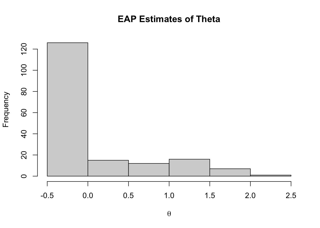
## EAP Estimates of Latent Variables
```{r}
#| eval: true
hist(modelIRT_2PL_SI_samples$summary(variables = c("theta"))$mean,
     main="EAP Estimates of Theta",
     xlab = expression(theta))
```
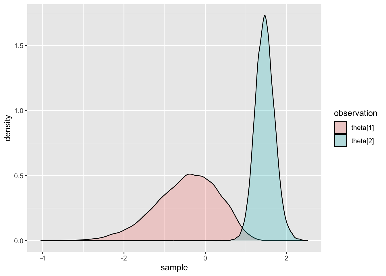
## Comparing Two Posterior Distributions
```{r}
#| eval: true
# Comparing Two Posterior Distributions
theta1 = "theta[1]"
theta2 = "theta[2]"
thetaSamples = modelIRT_2PL_SI_samples$draws(variables = c(theta1, theta2), format = "draws_matrix")
thetaVec = rbind(thetaSamples[,1], thetaSamples[,2])
thetaDF = data.frame(observation = c(rep(theta1,nrow(thetaSamples)), rep(theta2, nrow(thetaSamples))),
                     sample = thetaVec)
names(thetaDF) = c("observation", "sample")
ggplot(thetaDF, aes(x=sample, fill=observation)) +geom_density(alpha=.25)
```
## Comparing EAP Estimates with Posterior SDs
```{r}
#| eval: true
plot(y = modelIRT_2PL_SI_samples$summary(variables = c("theta"))$sd,
     x = modelIRT_2PL_SI_samples$summary(variables = c("theta"))$mean,
     xlab = "E(theta|Y)", ylab = "SD(theta|Y)", main="Mean vs SD of Theta")
```
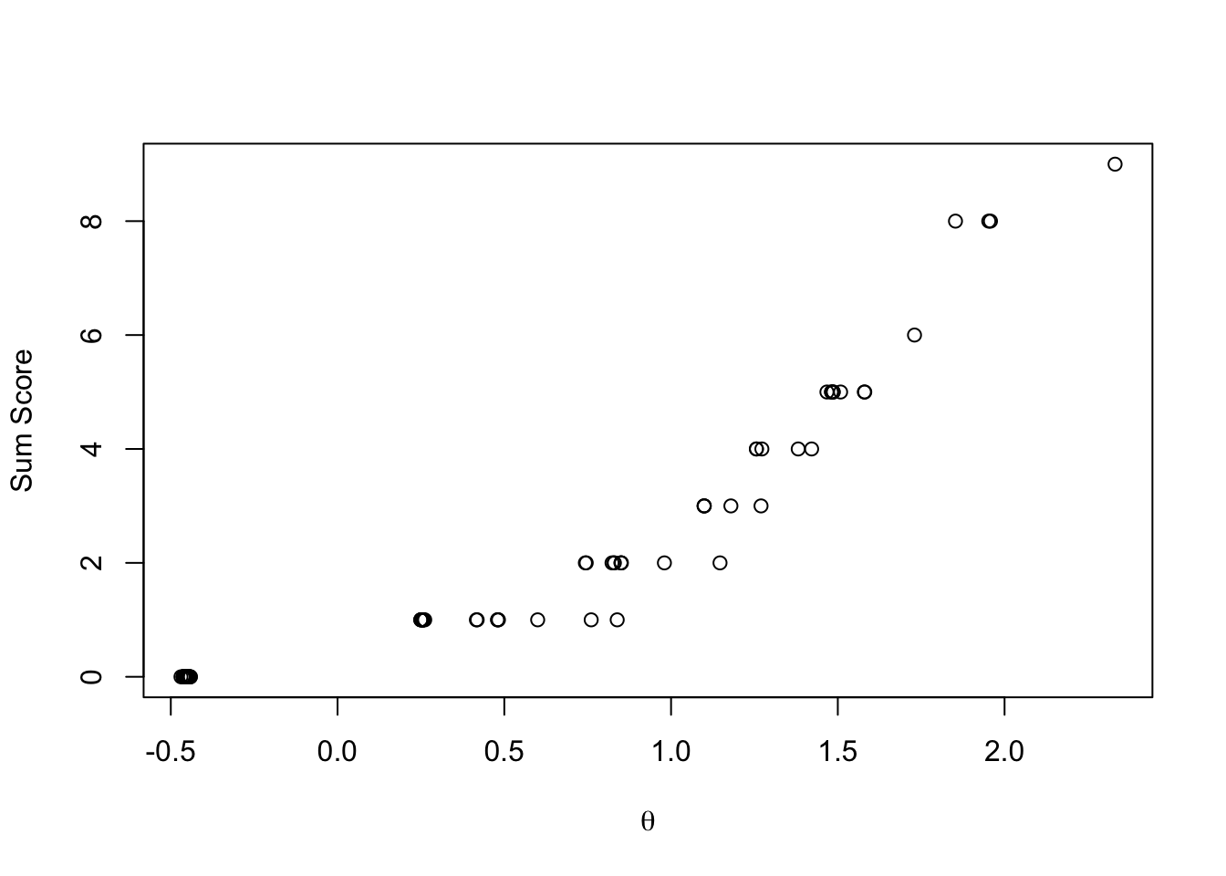
## Comparing EAP Estimates with Sum Scores
```{r}
#| eval: true
plot(y = rowSums(conspiracyItemsDichtomous),
     x = modelIRT_2PL_SI_samples$summary(variables = c("theta"), .cores = 4)$mean,
     ylab = "Sum Score", xlab = expression(theta))
```
## Extension: Factor Score
1. Thurston's Regression Method
2. Bartlett's Method (maximum-likelihood)
3. Bayesian approach
See more on my [website](https://jihongzhang.org/posts/2024-03-12-Factor-Score-Sum-Score-Reliability/)
## Next Class
- Discrimination/Difficulty Parameterization
## Resources
- [Dr. Templin's slide](https://jonathantemplin.github.io/Bayesian-Psychometric-Modeling-Course-Fall2022/lectures/lecture04b/04b_Modeling_Observed_Data#/title-slide)