Example 01: Make Friends with R

1 How to use this file

1. To test a certain chunk of code, click the “Copy” icon in the lower right corner of the chunk block (see screenshot below)

   • 

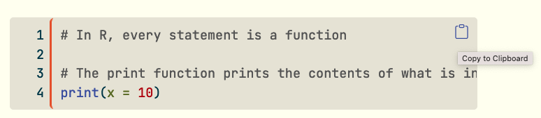
   • Try copying the following code

     a = 1 + 1
     b = a + 1
     print(b)

2 Getting Started with R

2.1 What is R?

R is a powerful programming language and environment specifically designed for statistical computing and graphics. It’s free, open-source, and has a vast ecosystem of packages for data analysis, visualization, and machine learning.

• Free and Open Source: No licensing costs
• Extensive Package Ecosystem: Over 18,000 packages available
• Excellent for Statistics: Built by statisticians, for statisticians
• Great Visualization: ggplot2 and other packages for beautiful graphics
• Reproducible Research: R Markdown and Quarto for literate programming
• Active Community: Large, helpful community of users

2.2 R vs RStudio

• R: The programming language and computing environment

  

• RStudio: An integrated development environment (IDE) that makes R easier to use

  

2.3 RStudio Interface Layout

RStudio organizes an analysis into four main panes. Knowing where each task belongs makes it easier to separate saved code, temporary output, data objects, and files.

• Source (top-left): Write and save .R scripts and Quarto documents.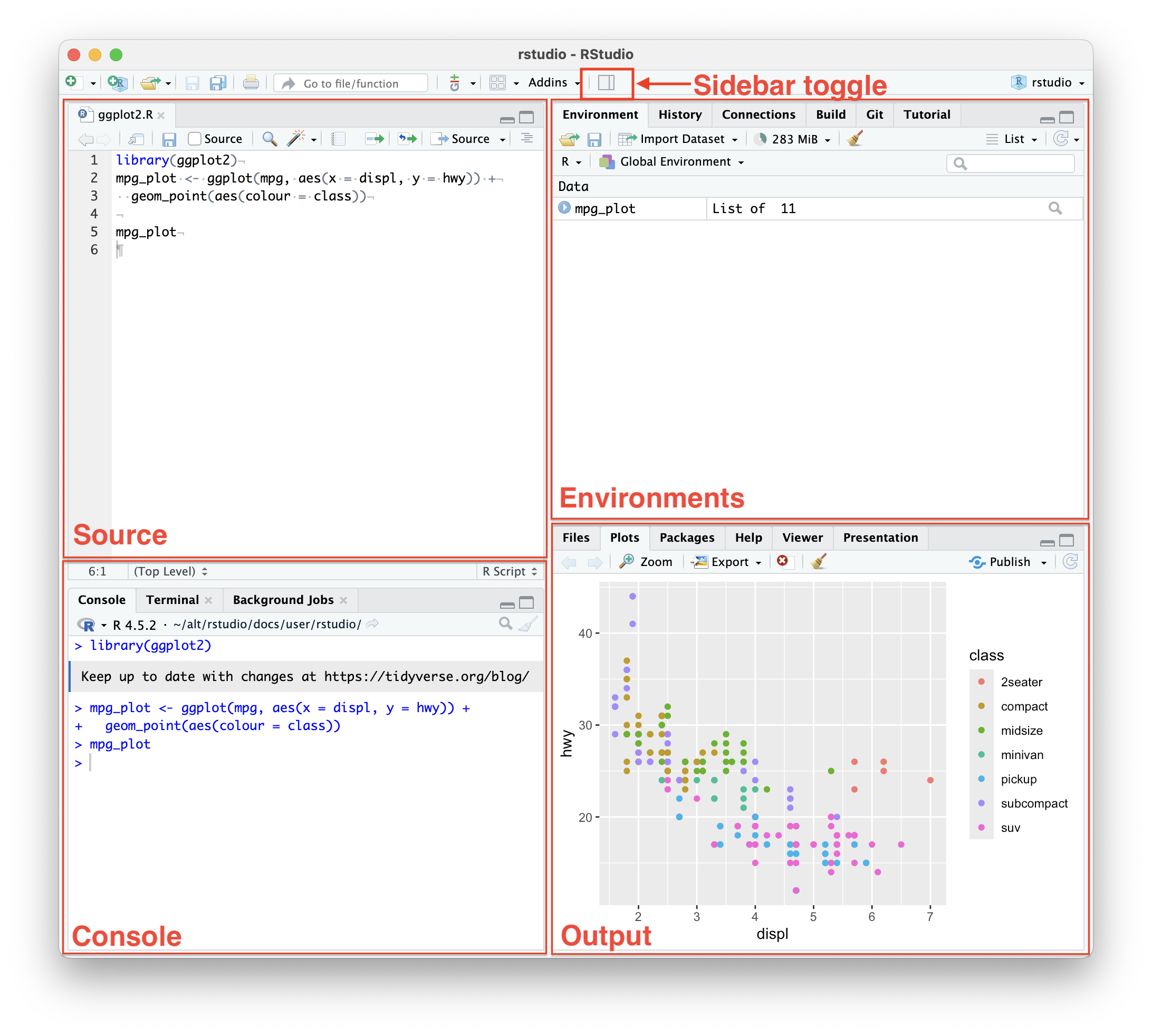
• Console (bottom-left): Run commands and review messages, warnings, and errors.
• Environment/History (top-right): Inspect objects created during the current R session and review previously executed commands.
• Files/Plots/Packages/Help (bottom-right): Navigate project files, inspect figures, manage packages, and read documentation.

RStudio’s four-pane layout, including the Source, Console, Environment, and Output areas.

Screenshot source: Posit RStudio User Guide: Pane Layout.

2.3.1 A Basic RStudio Workflow

Use the Projects menu to create a new RStudio Project or open an existing one.

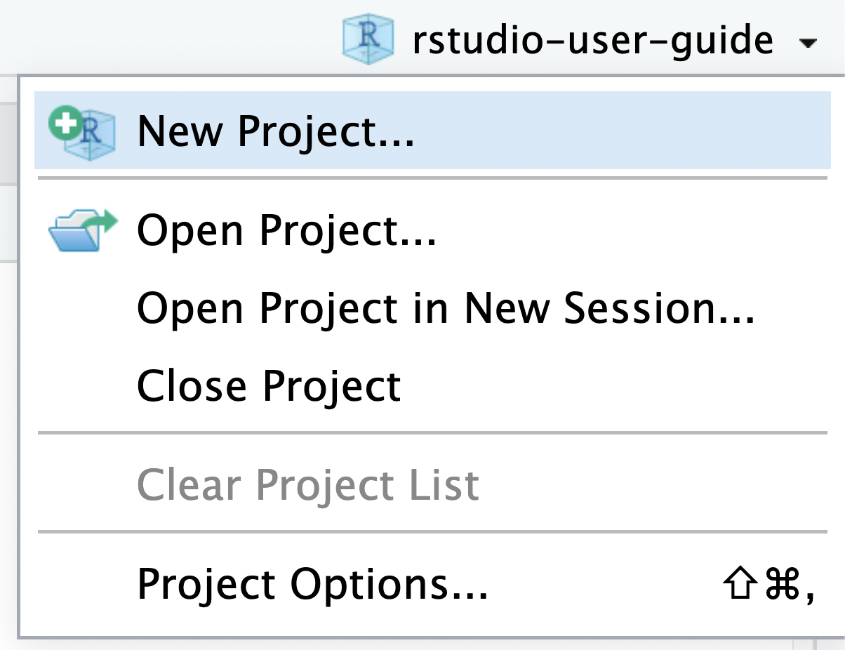
Screenshot source: Posit RStudio User Guide: RStudio Projects.

1. Create or open an RStudio Project for the analysis.
2. Write commands in an .R script rather than relying only on the Console.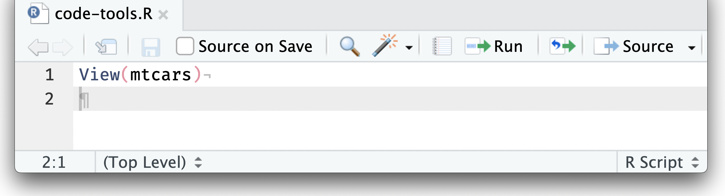
3. Run the current line or selected code with Ctrl+Enter (Cmd+Enter on Mac).
4. Inspect created objects in the Environment pane and figures in the Plots pane.
5. Save the script so another person can rerun and verify the analysis.

Use the Run button or Ctrl+Enter to execute code from an R script.

Screenshot source: Posit RStudio User Guide: Executing Code.

3 Suggestion in R

# R comments begin with a # -- there are no multiline comments

# RStudio helps you build syntax
#   GREEN: Comments and character values in single or double quotes
#   BLUE: Functions and keywords
#   BLACK: Variable names and values

# You can use the tab key to complete object names, functions, and arguments

# R is case sensitive. That means R and r are two different things.

# Good naming conventions:
#   - Use descriptive names: my_data instead of x
#   - Use underscores or dots: my_data or my.data
#   - Avoid spaces and special characters (except . and _)
#   - Don't start with numbers: 1data is invalid, data1 is valid


## Install the packages used in this tutorial once per computer
install.packages(
  c("dplyr", "ggplot2", "haven", "here", "psych", "readr", "tidyr")
)

4 Basic Data Types in R

# R has several basic data types:

# 1. Numeric (double) - decimal numbers
numeric_value <- 3.14
class(numeric_value)

# 2. Integer - whole numbers
integer_value <- 42L  # The L suffix makes it an integer
class(integer_value)

# 3. Character (string) - text
character_value <- "Hello, R!"
class(character_value)

# 4. Logical (boolean) - TRUE/FALSE
logical_value <- TRUE
class(logical_value)

# 5. Complex - complex numbers
complex_value <- 3 + 4i
class(complex_value)

# Check the type of any object
typeof(numeric_value)
is.numeric(numeric_value)
is.character(character_value)

5 R Functions

# In R, every statement is a function

# The print function prints the contents of what is inside to the console
print(x = 10)

# The terms inside the function are called the arguments; here print takes x
#   To find help with what the arguments are use:
?print

# Each function returns an object
print(x = 10)

# You can determine what type of object is returned by using the class function
class(print(x = 10))

# Function syntax: function_name(argument1, argument2, ...)
# Examples of common functions:
sqrt(16)           # Square root
abs(-5)            # Absolute value
round(3.14159, 2)  # Round to 2 decimal places
length(c(1,2,3,4)) # Length of a vector
sum(c(1,2,3,4))    # Sum of values
mean(c(1,2,3,4))   # Mean of values

6 Getting Help

# R has excellent help documentation
?mean                    # Help for a function
??"regression"          # Search for functions containing "regression"
help(mean)              # Same as ?mean
example(mean)           # Run examples for a function

# Online resources:
# - R Documentation: https://www.rdocumentation.org/
# - Stack Overflow: https://stackoverflow.com/questions/tagged/r
# - R-bloggers: https://www.r-bloggers.com/
# - RStudio Community: https://community.rstudio.com/

# Installing and loading packages
install.packages("package_name")  # Install once
library(package_name)             # Load each session
require(package_name)             # Alternative to library()

7 Vectors - The Building Blocks

Vectors are the most basic data structure in R. They are one-dimensional arrays that can contain multiple elements of the same type (e.g., all numbers, all text, or all logical values).

7.1 Creating Vectors

# Use the c() function (combine) to create vectors
numeric_vector <- c(1, 2, 3, 4, 5)
character_vector <- c("apple", "banana", "cherry")
logical_vector <- c(TRUE, FALSE, TRUE)

# Display the vectors
numeric_vector
character_vector
logical_vector

7.2 Named Vectors

A named vector associates each value with a descriptive label. Names make it possible to retrieve values by label instead of only by position.

# Store the mean outcome for each experimental condition
condition_means <- c(
  control = 72.4,
  online = 76.8,
  in_person = 81.2
)

# Display the complete named vector
condition_means

# Retrieve a value by its name
condition_means["in_person"]

# Inspect the vector's names
names(condition_means)

The names are labels attached to the values; they do not change the vector’s underlying numeric data type.

7.3 Creating Sequences

# Using the colon operator for simple sequences
sequence <- 1:10
sequence

# You can also create descending sequences
10:1

7.4 Using seq() for More Control

# seq() gives you more control over sequences
# Create a sequence from 1 to 10, incrementing by 2
seq(from = 1, to = 10, by = 2)

# Create a sequence with exactly 5 equally-spaced values between 1 and 10
seq(1, 10, length.out = 5)

7.5 Repeating Values with rep()

# Repeat a single value multiple times
rep(5, times = 3)

# Repeat an entire vector multiple times
rep(c(1, 2), times = 3)

# Repeat each element multiple times before moving to the next
rep(c(1, 2), each = 3)

7.6 Vector Operations

# R performs operations element-wise on vectors
x <- c(1, 2, 3, 4, 5)
y <- c(10, 20, 30, 40, 50)

# Element-wise addition
x + y

# Element-wise multiplication
x * y

# Element-wise exponentiation
x^2

# You can also perform operations with a single value (vectorization)
x + 10
x * 2

8 Categorical/Factor Vectors (Factors)

Factors are used for categorical variables in R. They store both the values and the levels (categories), which is essential for statistical analysis and plotting. R uses factors to understand categorical variables properly.

8.1 Creating Basic Factors

# Create a factor from a character vector
gender <- c("Male", "Female", "Male", "Female", "Male")
gender_factor <- factor(gender)
gender_factor

# Check the levels (categories)
levels(gender_factor)

# See how many observations in each category
table(gender_factor)

8.2 Creating Factors with Specific Levels

# You can specify the order of levels explicitly
# This is useful when you want a specific order for plotting or analysis
education <- c("High School", "College", "Graduate", "High School")
education_factor <- factor(education,
                          levels = c("High School", "College", "Graduate"))
education_factor

# View the levels in the order you specified
levels(education_factor)

8.3 Ordered Factors (Ordinal Data)

# Use ordered = TRUE for ordinal data (categories with a meaningful order)
satisfaction <- c("Low", "Medium", "High", "Medium", "Low")
satisfaction_ordered <- factor(satisfaction,
                               levels = c("Low", "Medium", "High"),
                               ordered = TRUE)
satisfaction_ordered

# Notice the < signs indicating the order
print(satisfaction_ordered)

The distinction between unordered and ordered factors determines which comparisons and statistical models are appropriate in practice.

Scenario	Variable	Factor type	How it is used
Experimental conditions	Control, Online, In-person	Unordered	Compare each treatment group without assuming a ranking
Geographic region	North, South, East, West	Unordered	Estimate differences among categories without imposing an order
Satisfaction	Dissatisfied, Neutral, Satisfied	Ordered	Examine whether responses tend toward higher satisfaction
Disease severity	Mild, Moderate, Severe	Ordered	Model the probability of being in a higher severity category
Education	High school, Bachelor’s, Master’s, Doctorate	Ordered	Preserve the educational ranking without assuming equal distances between levels

8.4 Factor Operations and Summaries

# Get frequency counts
table(gender_factor)

8.5 Converting Between Data Types

# Convert factor back to character
as.character(gender_factor)

# Convert to numeric (gives you the underlying level numbers, not always useful)
as.numeric(gender_factor)

# Be careful: converting numeric to factor
age_values <- c(25, 30, 35, 25, 40, 30)
age_factor <- factor(age_values)
age_factor  # Notice it treats each unique number as a separate category

8.6 Grouping Continuous Data into Categories

8.6.1 Method 1: Using cut() Function

# cut() is ideal for dividing continuous data into intervals
ages <- c(22, 25, 30, 35, 40, 45, 50, 55, 60, 65)

age_categories <- cut(ages,
                      breaks = c(0, 30, 50, 100),  # Define the breakpoints
                      labels = c("Young", "Middle", "Senior"),  # Label each interval
                      include.lowest = TRUE)  # Include the lowest value in the first interval
age_categories

# Check the distribution
table(age_categories)

8.6.2 Method 2: Using ifelse() for Custom Grouping

# ifelse() gives you more control over custom conditions
ages <- c(22, 25, 30, 35, 40, 45, 50, 55, 60, 65)

age_groups_custom <- ifelse(ages < 30, "Young",
                            ifelse(ages < 50, "Middle", "Senior"))

# Convert to an ordered factor
age_groups_factor <- factor(age_groups_custom,
                            levels = c("Young", "Middle", "Senior"),
                            ordered = TRUE)
age_groups_factor

# View the distribution
table(age_groups_factor)
summary(age_groups_factor)

8.7 Why Use Factors?

Factors are essential because they:

• Help R recognize categorical data in statistical models (e.g., ANOVA, regression)
• Control the order of categories in plots and tables
• Store data more efficiently than character strings
• Prevent typos from creating unintended new categories

9 R Objects

# Each object can be saved into the R environment (the workspace here)
#   You can save the results of a function call to a variable of any name
MyObject = print(x = 10)
class(MyObject)

# You can view the objects you have saved in the Environment tab in RStudio
# Or type their name
MyObject

# There are literally thousands of types of objects in R (you can create them),
#   but for our course we will mostly be working with data frames (more later)

# The process of saving the results of a function to a variable is called
#   assignment. There are several ways you can assign function results to
#   variables:

# The equals sign takes the result from the right-hand side and assigns it to
#   the variable name on the left-hand side:
MyObject = print(x = 10)

# The <- (Alt "-" in RStudio) functions like the equals (right to left)
MyObject2 <- print(x = 10)

identical(MyObject, MyObject2)

# The -> assigns from left to right:
print(x = 10) -> MyObject3

identical(MyObject, MyObject2, MyObject3)

# Best practice: Use <- for assignment (more explicit)
# Use = only for function arguments

10 Working with Data Structures

10.1 Lists

# Lists can contain elements of different types
my_list <- list(
  name = "John",
  age = 30,
  scores = c(85, 90, 78),
  passed = TRUE
)

# Accessing list elements
my_list$name
my_list[["age"]]
my_list[[3]]

# Lists are very flexible and useful for complex data structures

10.2 Matrices

# Matrices are 2-dimensional arrays with the same data type
my_matrix <- matrix(1:12, nrow = 3, ncol = 4)
my_matrix

# Creating matrices from vectors
matrix(c(1,2,3,4,5,6), nrow = 2, ncol = 3)

# Matrix operations
matrix1 <- matrix(1:4, nrow = 2)
matrix2 <- matrix(5:8, nrow = 2)
matrix1 + matrix2
matrix1 * matrix2  # Element-wise multiplication

11 Importing and Exporting Data

A data frame stores rectangular data: each row represents an observation or case, and each column represents a variable. Importing data is not only a file-opening task. You must also verify that the software interpreted the rows, columns, missing values, and variable types correctly.

11.1 Organize the Project Before Importing

For this exercise, create an RStudio Project in the folder containing your script and the two practice data files. Keep raw data separate from exported results.

experiment-design-practice/
├── experiment-design-practice.Rproj
├── MakeFriendsWithR.R
├── heights.csv
├── wide.sav
└── outputs/

The here::here() function builds paths from the project root, which makes the same script easier to run on Windows, macOS, and Linux. Avoid setwd() and computer-specific absolute paths in code that others need to reproduce.

here::here()
list.files(here::here())

11.2 Import a CSV with RStudio

1. Select File → Import Dataset → From Text (readr), or select Import Dataset in the Environment pane.
2. Select heights.csv and inspect the data preview, variable names, delimiter, missing-value settings, and inferred variable types.
3. Review the Code Preview, then select Import.
4. Copy the generated code into your .R script so the import can be reproduced.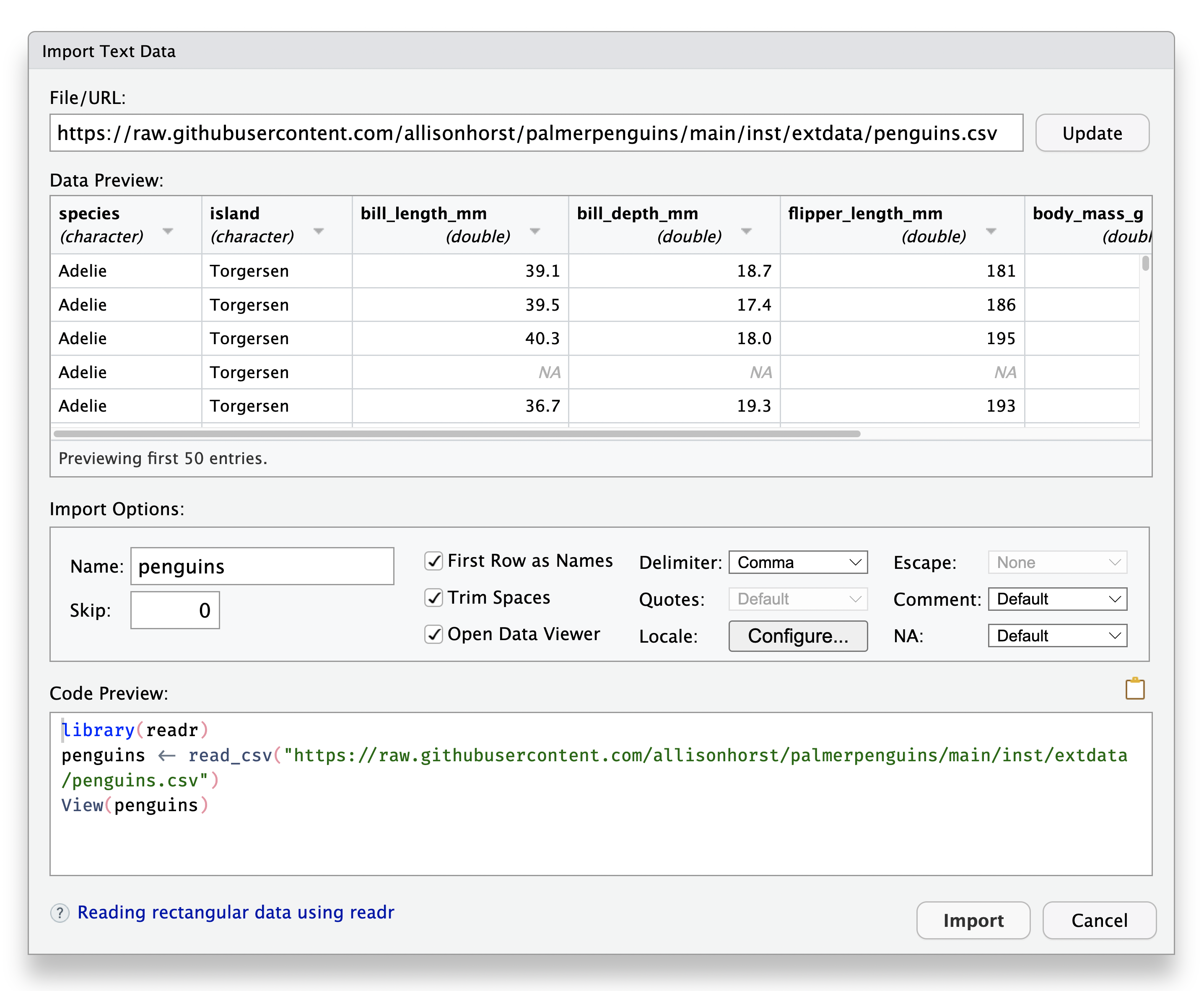

RStudio’s Import Text Data wizard previews the data, import settings, and generated R code.

Screenshot source: Posit RStudio User Guide: Local Data.

11.3 Import the Same CSV with Code

The scripted import is the reproducible record of the choices made in the import window.

heights_data <- readr::read_csv(
  file = here::here("heights.csv"),
  show_col_types = FALSE
)

heights_data

Base R provides an alternative:

heights_data_base <- read.csv(
  file = here::here("heights.csv"),
  stringsAsFactors = FALSE
)

11.4 Import an SPSS File

The haven package imports SPSS .sav files and preserves useful metadata such as variable and value labels.

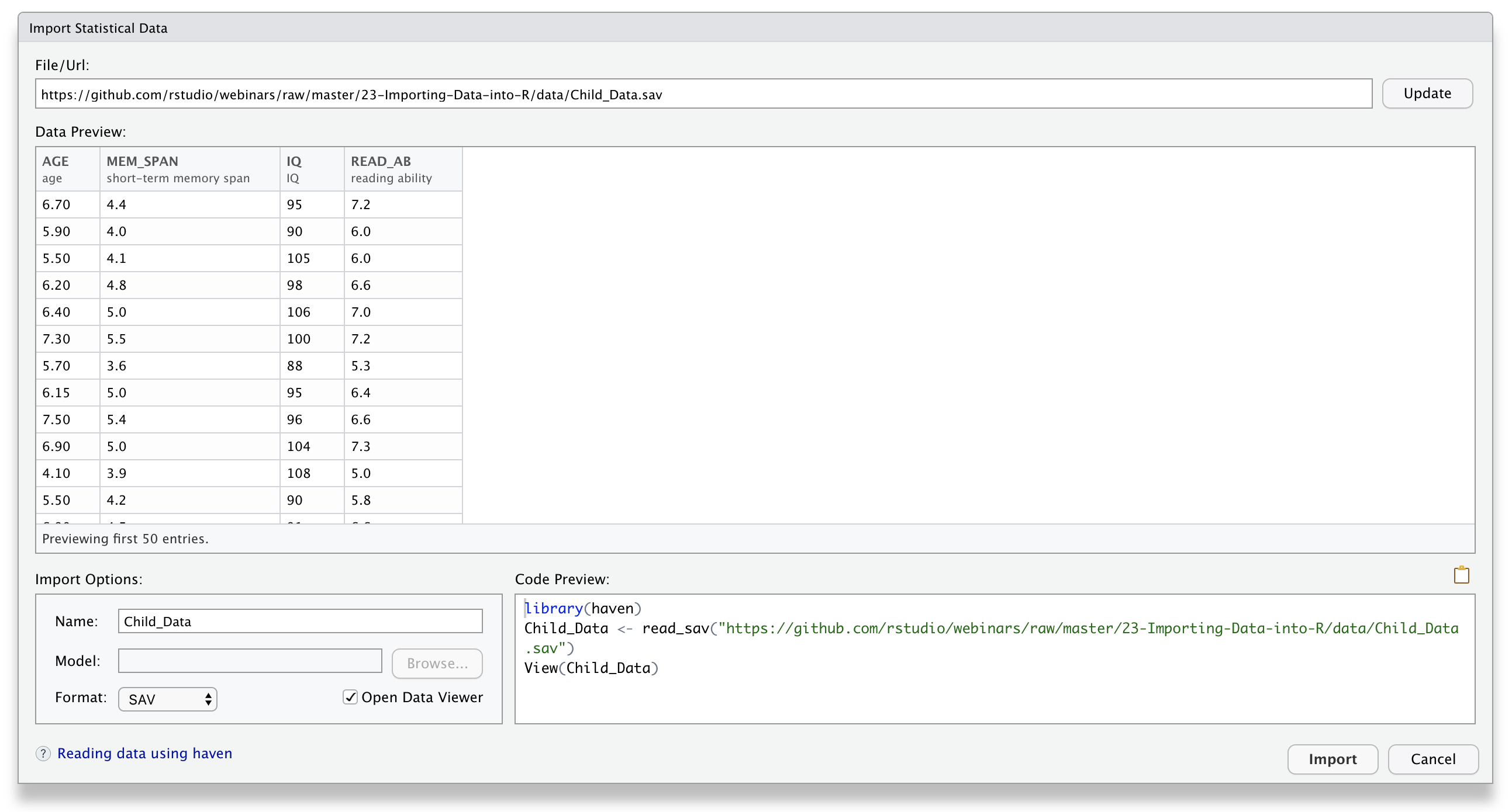
RStudio’s Import Statistical Data dialog previews an SPSS file and displays the corresponding haven code.

Screenshot source: Posit Support: Importing Data with the RStudio IDE.

wide_data <- haven::read_sav(
  file = here::here("wide.sav")
)

wide_data

Note

Labels imported from SPSS are metadata, not a guarantee that a variable has the correct measurement level or coding. Verify the codebook, value labels, missing-value definitions, and experimental-unit identifier before analysis.

11.5 Inspect Data After Import

Use View() or select a data-frame object in the Environment pane to open RStudio’s spreadsheet-like Data Viewer.

dplyr::glimpse(heights_data)
summary(heights_data)
colSums(is.na(heights_data))
View(heights_data)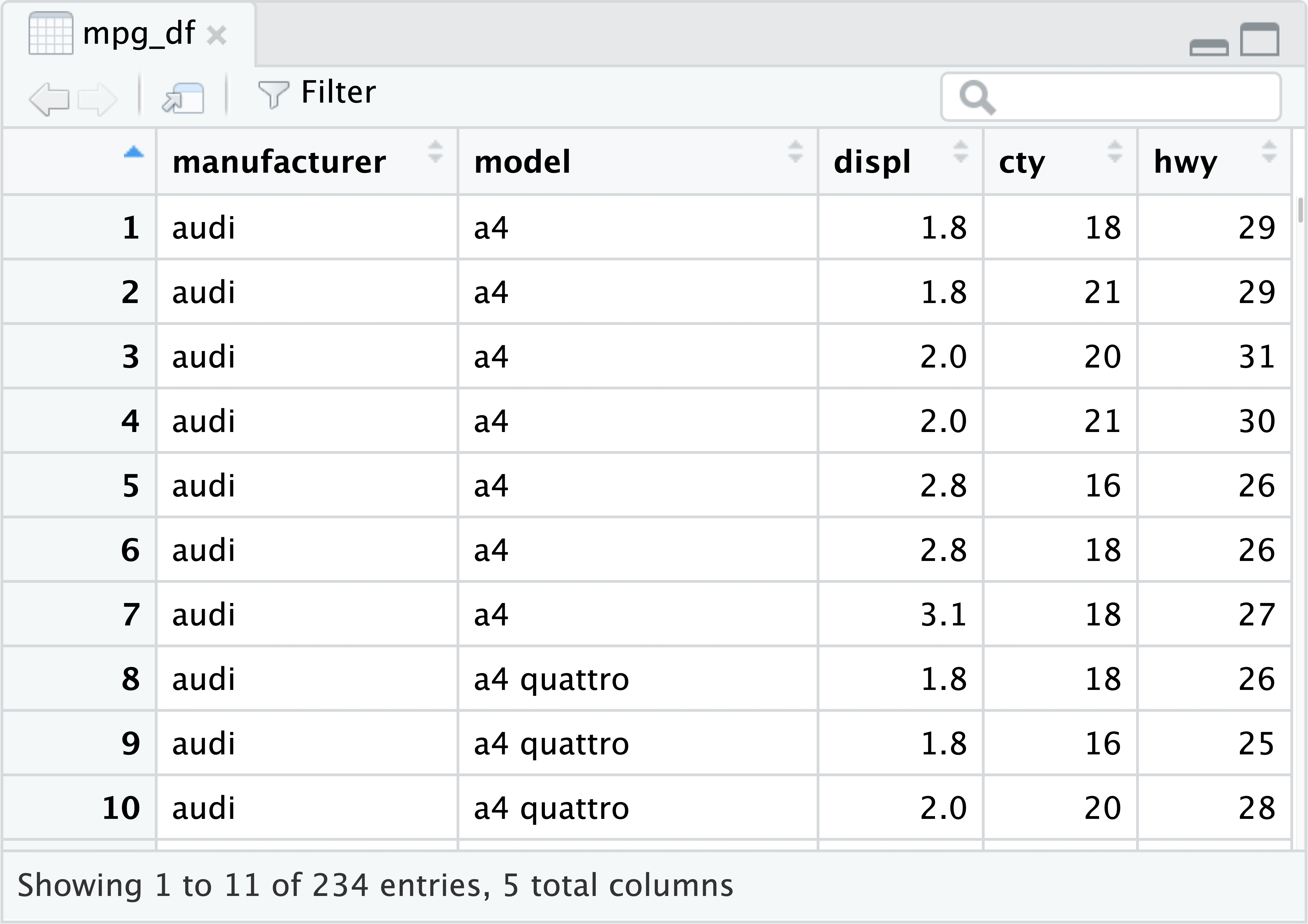

The RStudio Data Viewer supports sorting, filtering, and searching while inspecting imported data.

After every import, check at least the following:

• The number of rows and columns matches expectations.
• The experimental-unit identifier is present and unique when it should be.
• Numeric, categorical, date, and text variables have appropriate types.
• Missing values use the intended codes rather than values such as -99 or blank strings.
• Treatment labels and factor levels match the study design and codebook.

Warning

Sorting or filtering in the Data Viewer changes only the display. Record all substantive data transformations in the script.

Screenshot source: Posit RStudio User Guide: Data Viewer.

11.6 Export Data Reproducibly

Keep the original files unchanged. Write cleaned or transformed data to a separate outputs folder with informative file names.

output_dir <- here::here("outputs")
dir.create(output_dir, showWarnings = FALSE)

# CSV is portable across statistical software.
readr::write_csv(
  heights_data,
  file = file.path(output_dir, "heights-clean.csv"),
  na = ""
)

# SPSS preserves a workflow for collaborators who use .sav files.
haven::write_sav(
  wide_data,
  path = file.path(output_dir, "wide-clean.sav")
)

# RDS preserves R-specific classes and attributes.
saveRDS(
  object = list(heights = heights_data, wide = wide_data),
  file = file.path(output_dir, "imported-data.rds")
)

list.files(output_dir)

• Use CSV for portable rectangular data.
• Use SPSS when collaborators need labels and .sav compatibility.
• Use RDS when another R analysis must preserve classes and attributes.

After exporting, reopen the saved file and verify its dimensions, variable names, types, missing values, and labels before sharing or analyzing it.

12 Working with Data Frames

# Data frames are the most common data structure for statistical analysis
# They are like spreadsheets with rows (observations) and columns (variables)

# Basic data frame operations
dim(heights_data)        # Dimensions (rows, columns)
nrow(heights_data)       # Number of rows
ncol(heights_data)       # Number of columns
names(heights_data)      # Column names
str(heights_data)        # Structure of the data frame
head(heights_data)       # First 6 rows
tail(heights_data)       # Last 6 rows
summary(heights_data)    # Summary statistics

# Accessing data frame elements
heights_data[1, 2]       # Row 1, Column 2
heights_data[1:5, ]      # Rows 1-5, all columns
heights_data[, "ID"]     # All rows, column named "ID"
heights_data$ID          # Same as above (preferred method)

# Subsetting data frames
subset(heights_data, HeightIN > 70)
heights_data[heights_data$HeightIN > 70, ]

12.1 Exercise

• Obtain the following information from wide_data
  • Dimensions (rows, columns)
  • Number of rows
  • Number of columns
  • Column names
  • Structure of the data frame
  • First 6 rows
  • Last 6 rows
  • Summary statistics

Optional: Extended R Skills
The remaining sections cover optional extended R skills. They are useful for deeper practice but are not required for the core lesson.

13 Merging R data frame objects

# The wide_data and heights_data have the same set of ID numbers.
# We can use the merge() function to merge them into a single data frame.
# Here, x is the name of the left-side data frame and y is the name of the
# right-side data frame. The arguments by.x and by.y specify the variable(s)
# by which we will merge:
all_data <- merge(
  x = wide_data,
  y = heights_data,
  by.x = "ID",
  by.y = "ID"
)
all_data

## Method 2: Use dplyr method (the pipe operator |> can be typed using Ctrl+Shift+M on Windows or Cmd+Shift+M on Mac)
library(dplyr)
wide_data |>
  left_join(heights_data, by = "ID")

# Different types of joins:
# left_join(): Keep all rows from left table
# right_join(): Keep all rows from right table
# inner_join(): Keep only rows that appear in both tables
# full_join(): Keep all rows from both tables

14 Transforming Wide to Long

In wide format, repeated measurements occupy separate columns. pivot_longer() stacks those columns into a measurement column and a value column, producing multiple rows for each participant.

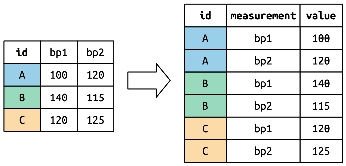
Wide data transformed into long data with pivot_longer(). The participant ID is repeated for each measurement. Source: R for Data Science (2e), Figure 5.3.

# Sometimes, certain packages require repeated measures data to be in a long
# format (where each measurement is on a separate row rather than in separate columns).

library(dplyr) # contains variable selection

## Wrong Way (pivoting DV and Age separately creates unwanted combinations)
all_data_long <- all_data |>
  tidyr::pivot_longer(starts_with("DVTime"), names_to = "DV", values_to = "DV_Value") |>
  tidyr::pivot_longer(starts_with("AgeTime"), names_to = "Age", values_to = "Age_Value")

one_person <- all_data_long  |>
  filter(ID == "1")

one_person

## Correct Way (pivot both variables together, then separate and widen properly)
all_data_long <- all_data |>
  tidyr::pivot_longer(c(starts_with("DVTime"), starts_with("AgeTime"))) |>
  tidyr::separate(name, into = c("Variable", "Time"), sep = "Time") |>
  tidyr::pivot_wider(names_from = "Variable", values_from = "value")

one_person <- all_data_long |>
  filter(ID == "1")
one_person

# Understanding data reshaping:
# Wide format: Each time point has its own column
# Long format: Time points are in rows, with a time variable

14.1 Exercise

14.1.1 Practice: Wide to Long with dplyr

In this exercise, you will practice reshaping repeated-measures data from wide format to long format using a dplyr pipeline (with tidyr functions).

1. Create the small wide data frame shown below.
2. Reshape it to long format so that you have four columns: id, time, dv, and age.
3. Compute the mean of dv by time as a verification step.

# Load packages
library(dplyr)
library(tidyr)

# 1) Start from a small wide toy data set
toy_wide <- tibble::tribble(
  ~id, ~dv_time1, ~dv_time2, ~dv_time3, ~age_time1, ~age_time2, ~age_time3,
   1,        10,        12,        15,         20,         21,         22,
   2,         8,        11,        11,         19,         20,         21,
   3,        14,        13,        16,         21,         22,         23
)

# 2) YOUR TURN: Convert to long using a single dplyr pipeline
#    Goal columns: id, time (1/2/3), dv, age
#    Hints:
#      - Use pivot_longer() on both dv_ and age_ columns together
#      - Separate the column name into variable (dv/age) and time (1/2/3)
#      - Use pivot_wider() to spread variable back into dv and age columns

14.1.1.1 Optional solution

toy_long <- toy_wide |>
  pivot_longer(
    cols = c(starts_with("dv_"), starts_with("age_")),
    names_to = "name",
    values_to = "value"
  ) |>
  separate(name, into = c("variable", "time"), sep = "_time") |>
  pivot_wider(names_from = variable, values_from = value) |>
  mutate(time = as.integer(time))

toy_long

toy_long |>
  group_by(time) |>
  summarize(mean_dv = mean(dv, na.rm = TRUE), .groups = "drop")

15 Data Manipulation with dplyr

# The dplyr package provides an intuitive set of functions for data manipulation

# Select columns
all_data |>
  select(ID, starts_with("DV"))

# Filter rows
all_data |>
  filter(ID < 5)

# Arrange rows
all_data |>
  arrange(ID)

# Create new variables
all_data |>
  mutate(
    DV_avg = (DVTime1 + DVTime2 + DVTime3) / 3,
    DV_range = DVTime3 - DVTime1
  )

# Group and summarize
all_data_long |>
  group_by(Time) |>
  summarize(
    mean_DV = mean(DV, na.rm = TRUE),
    sd_DV = sd(DV, na.rm = TRUE),
    n = n()
  )

16 Gathering Descriptive Statistics

# The psych package provides convenient functions for computing descriptive statistics.
## If you haven't installed it yet, run: install.packages("psych")
library(psych)

# Use describe() to get comprehensive descriptive statistics for all variables:
descriptives_wide <- describe(all_data)
descriptives_wide

descriptives_long <- describe(all_data_long)
descriptives_long

# Use describeBy() to compute descriptive statistics separately for each group:
descriptives_long_id <- describeBy(all_data_long, group = all_data_long$ID)
descriptives_long_id

# Basic descriptive statistics without packages:
mean(all_data_long$DV, na.rm = TRUE)
median(all_data_long$DV, na.rm = TRUE)
sd(all_data_long$DV, na.rm = TRUE)
var(all_data_long$DV, na.rm = TRUE)
min(all_data_long$DV, na.rm = TRUE)
max(all_data_long$DV, na.rm = TRUE)
quantile(all_data_long$DV, probs = c(0.25, 0.5, 0.75), na.rm = TRUE)

17 Transforming Data

# You can transform data by creating new variables.
all_data_long$AgeC <- all_data_long$Age - mean(all_data_long$Age)

# You can also use functions to create new variables. Here we create new terms
#   using the function for significant digits:
all_data_long$AgeYear <- signif(x = all_data_long$Age, digits = 2)
all_data_long$AgeDecade <- signif(x = all_data_long$Age, digits = 1)
head(all_data_long)

# Common data transformations:
# Centering: subtract mean
# Standardizing: (x - mean) / sd
# Log transformation: log(x)
# Square root: sqrt(x)
# Recoding: ifelse(condition, value_if_true, value_if_false)

# Example: Create standardized variables
all_data_long$DV_z <- scale(all_data_long$DV)
all_data_long$Age_z <- scale(all_data_long$Age)

18 Basic Plotting

# R has excellent plotting capabilities

# Base R plotting
hist(all_data_long$DV, main = "Distribution of DV", xlab = "DV Values")
boxplot(DV ~ Time, data = all_data_long, main = "DV by Time")
plot(all_data_long$Age, all_data_long$DV, main = "DV vs Age")

# Using ggplot2 (more modern and flexible)
# If you have not install the package yet, type in install.packages("ggplot2")
library(ggplot2)

# Histogram
ggplot(all_data_long, aes(x = DV)) +
  geom_histogram(bins = 30) +
  labs(title = "Distribution of DV", x = "DV Values", y = "Count")

# Boxplot
ggplot(all_data_long, aes(x = Time, y = DV)) +
  geom_boxplot() +
  labs(title = "DV by Time")

# Scatter plot
ggplot(all_data_long, aes(x = Age, y = DV)) +
  geom_point() +
  geom_smooth(method = "lm") +
  labs(title = "DV vs Age")

hw0_feedback <- read.csv(here::here("teaching/2025-01-13-Experiment-Design/Lecture01", "hw0_feedback.csv"))
table(hw0_feedback$Feedback)

19 Control Structures

# Conditional statements (if-else)
x <- 10
if (x > 5) {
  print("x is greater than 5")
} else {
  print("x is less than or equal to 5")
}

## Alternative method using ifelse() function (vectorized)
ifelse(x > 5,
       print("x is greater than 5"),
       print("x is less than or equal to 5"))

# For loops (repeat code a specific number of times)
for (i in 1:5) {
  print(paste("Iteration", i))
}

# While loops (repeat code while a condition is TRUE)
i <- 1
while (i <= 5) {
  print(paste("While iteration", i))
  i <- i + 1
}

# Apply functions (more efficient and "R-like" than explicit loops)
numbers <- 1:10
sapply(numbers, function(x) x^2)  # Returns a vector
lapply(numbers, function(x) x^2)  # Returns a list

20 Working with Missing Data

# R uses NA (Not Available) to represent missing data
# Check for missing values in a variable
is.na(all_data_long$DV)              # Returns TRUE/FALSE for each value
sum(is.na(all_data_long$DV))        # Count the number of missing values
complete.cases(all_data_long)        # Check which rows have no missing data

# Remove rows that contain any missing data
all_data_long_complete <- na.omit(all_data_long)
# Alternative method (same result):
all_data_long_complete <- all_data_long[complete.cases(all_data_long), ]

# Replace missing values with the mean (simple imputation)
all_data_long$DV_imputed <- ifelse(
  is.na(all_data_long$DV),
  mean(all_data_long$DV, na.rm = TRUE),
  all_data_long$DV
)

21 Best Practices and Tips

# 1. Always use meaningful variable names
# 2. Comment your code
# 3. Use consistent formatting
# 4. Check your data after importing
# 5. Save your work regularly
# 6. Use version control (Git)
# 7. Write reproducible code
# 8. Use packages for common tasks
# 9. Learn to use help documentation
# 10. Practice regularly!

# Useful keyboard shortcuts in RStudio:
# Ctrl+Enter (Cmd+Enter on Mac): Run the current line or selected code
# Ctrl+Shift+Enter (Cmd+Shift+Enter on Mac): Run the entire script
# Ctrl+Shift+M (Cmd+Shift+M on Mac): Insert the pipe operator |>
# Ctrl+Shift+C (Cmd+Shift+C on Mac): Comment or uncomment selected lines
# Ctrl+Shift+R (Cmd+Shift+R on Mac): Insert a code section header