1 + 1[1] 2mean(c(1, 2, 3))[1] 2Welcome to your first steps in applied multivariate statistics! In this tutorial, you will learn how to use R and RStudio to run code, work with data, create plots, and support reproducible analyses.
Install R before installing RStudio. R performs the computations; RStudio provides the interface for working with R.
RStudio is designed specifically for R programming and organizes the tools needed for an analysis in one interface.
.R files.R scripts with syntax highlighting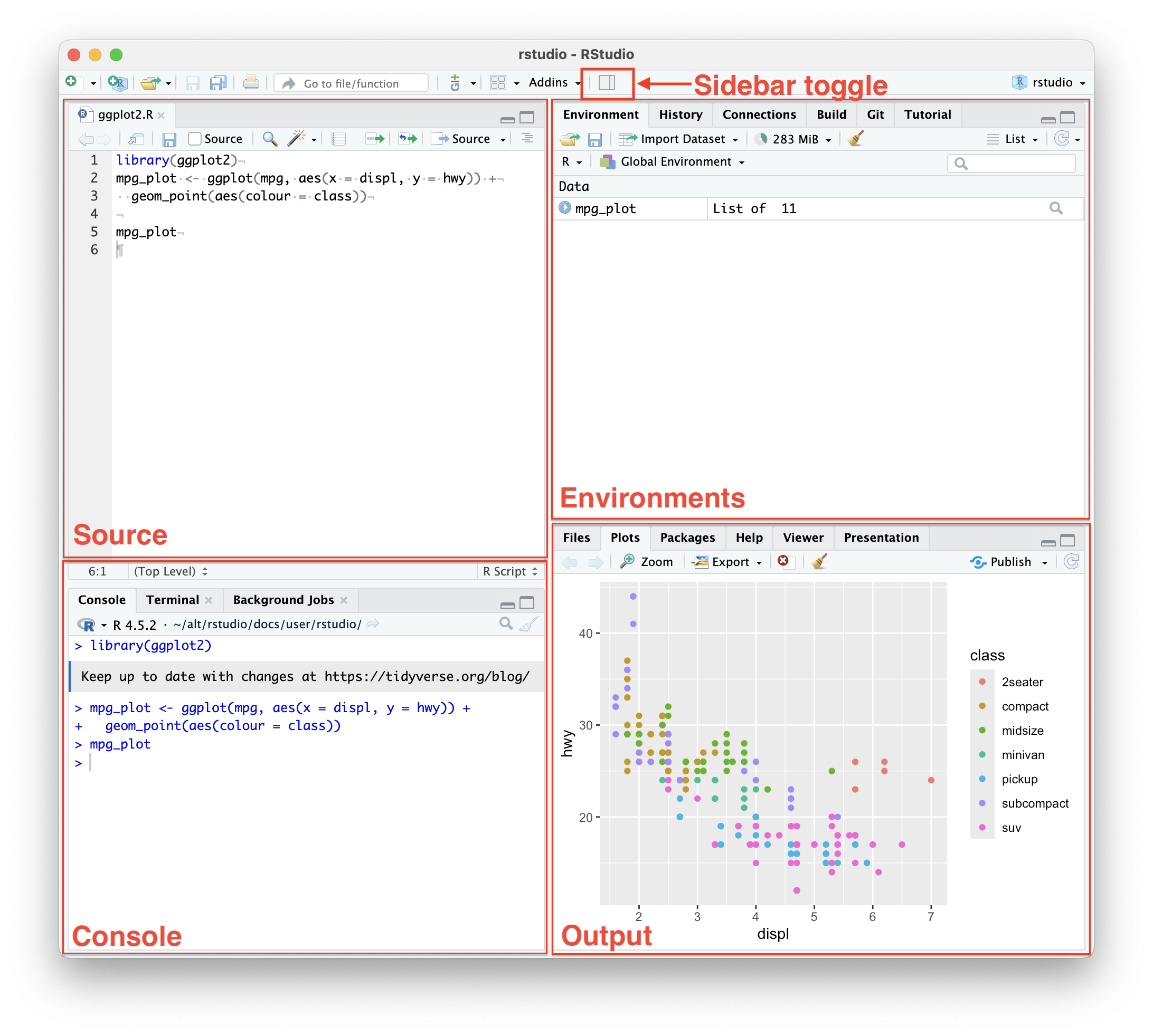
Screenshot source: Posit RStudio User Guide: Pane Layout.
.R script rather than relying only on the Console.You can run R commands directly in the Console, but an .R script creates a record that you can revise and rerun. Enter the following commands in a script, then run each line with Ctrl+Enter (Cmd+Enter on Mac):
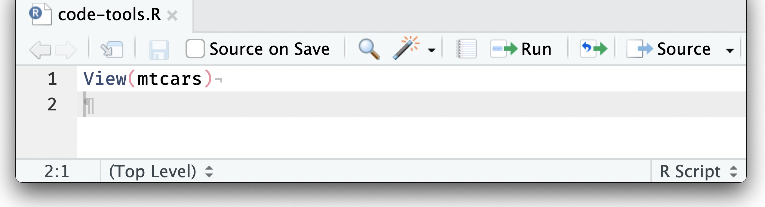
Screenshot source: Posit RStudio User Guide: Executing Code.
1 + 1[1] 2mean(c(1, 2, 3))[1] 2print("Hello, world!")install.packages() once per machine; load each time with library().install.packages(c("tidyverse", "readr", "ggplot2", "here"))library(tidyverse)── Attaching core tidyverse packages ──────────────────────── tidyverse 2.0.0 ──
✔ dplyr 1.2.0 ✔ readr 2.2.0
✔ forcats 1.0.1 ✔ stringr 1.6.0
✔ ggplot2 4.0.2 ✔ tibble 3.3.1
✔ lubridate 1.9.5 ✔ tidyr 1.3.2
✔ purrr 1.2.1
── Conflicts ────────────────────────────────────────── tidyverse_conflicts() ──
✖ dplyr::filter() masks stats::filter()
✖ dplyr::lag() masks stats::lag()
ℹ Use the conflicted package (<http://conflicted.r-lib.org/>) to force all conflicts to become errorslibrary(here)here() starts at /Users/jihong/Documents/Projects/website-jihongYou can also select Install in the Packages pane, enter the package names, and select Install in the dialog.
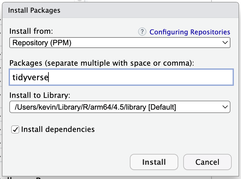
Screenshot source: Posit RStudio User Guide: Packages Pane.
readr::read_csv() for CSV; read.csv() is the base R alternative.heights.csv and inspect the data preview, variable names, and inferred data types..R script so the step is reproducible.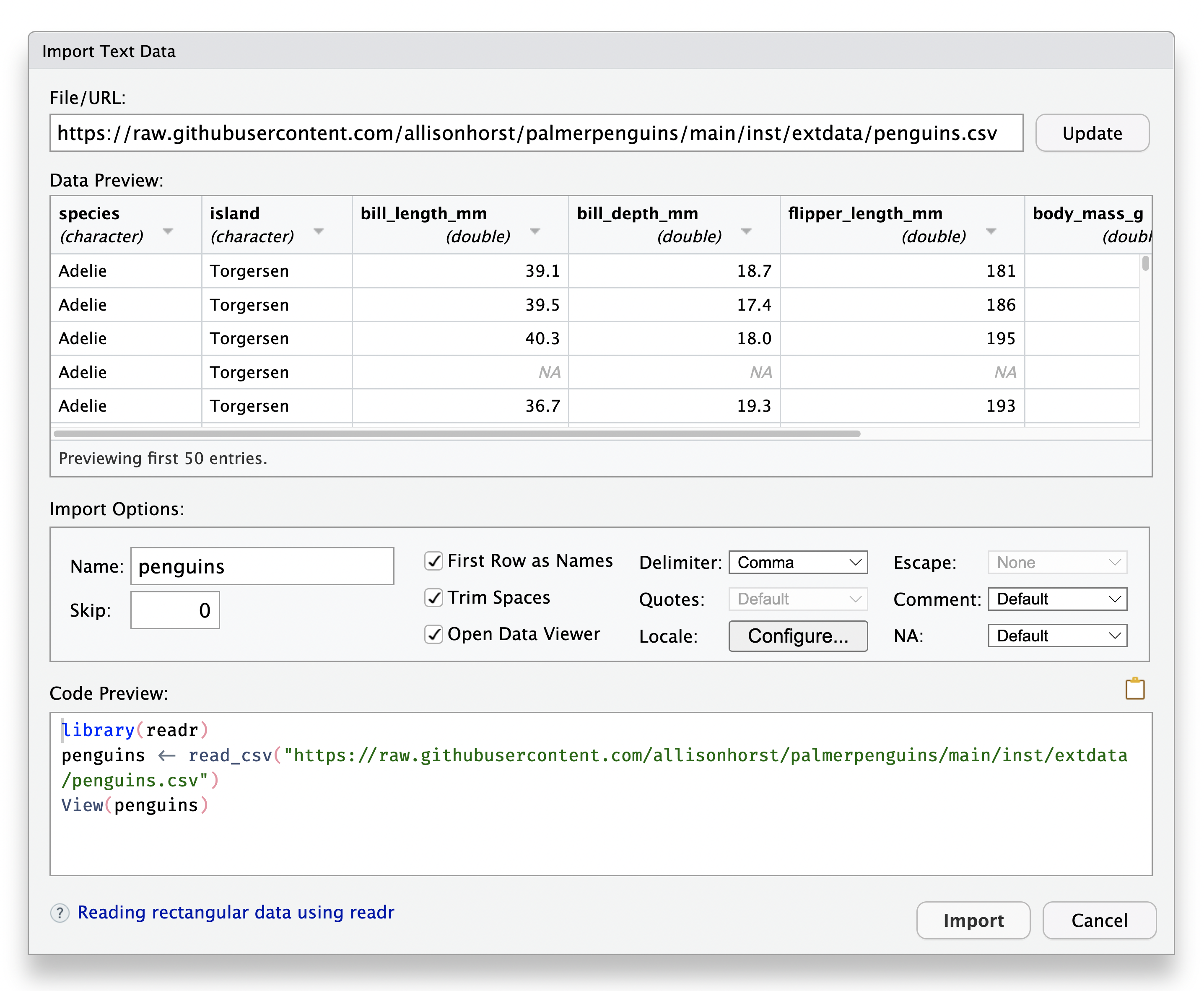
Screenshot source: Posit RStudio User Guide: Local Data.
Create a folder called data in your project folder, download heights.csv into it, and run one of the following commands:
# Read CSV with readr
height_data <- readr::read_csv(here::here("data", "heights.csv"))

# Base R alternative
height_data_base <- read.csv(here::here("data", "heights.csv"))Use View() or select a data-frame object in the Environment pane to open RStudio’s spreadsheet-like Data Viewer.
mpg_data <- ggplot2::mpg |>
  dplyr::select(manufacturer, model, displ, cty, hwy)

View(mpg_data)
In the Data Viewer, try these tasks:
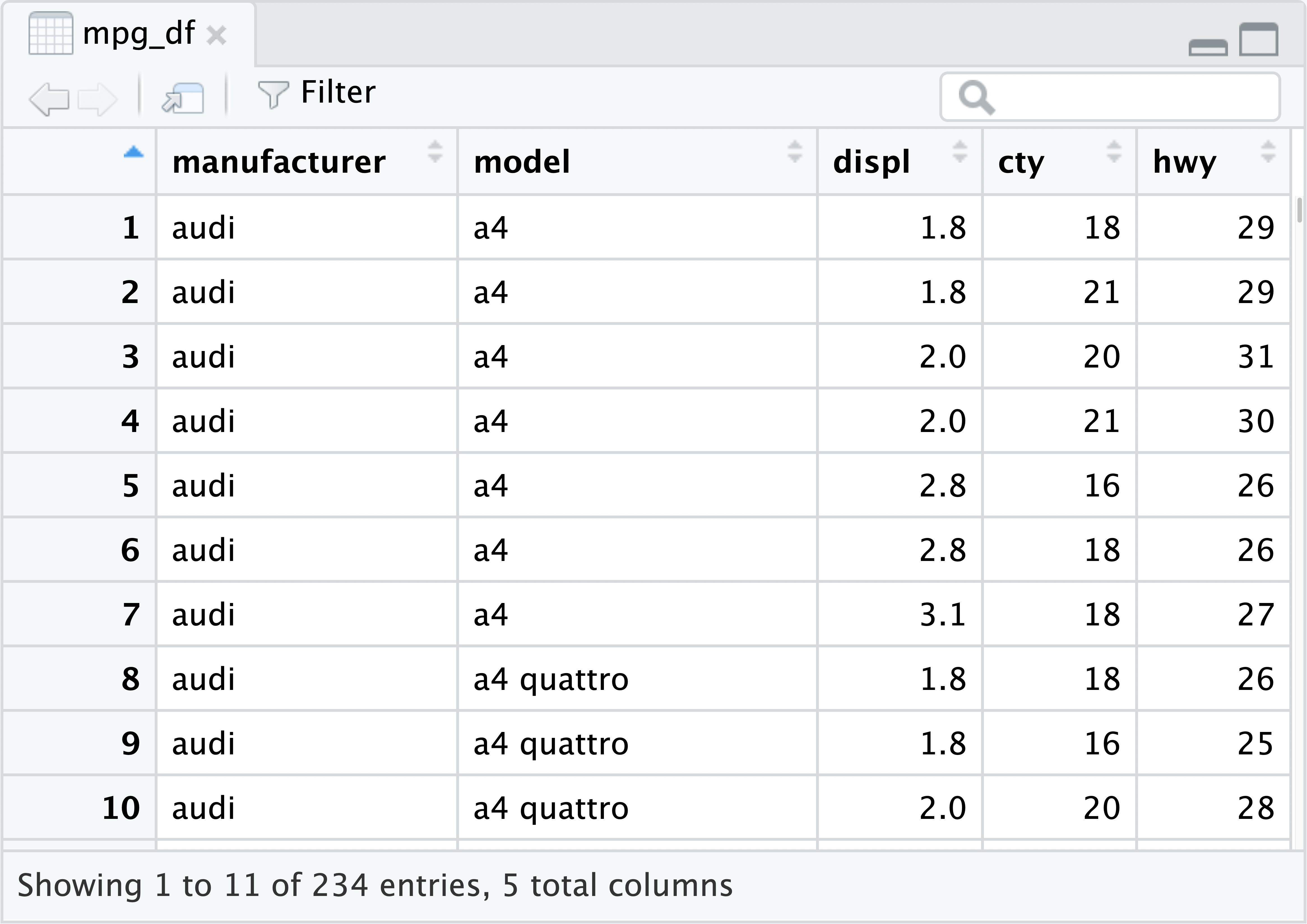
Sorting and filtering in the Data Viewer help you inspect the data, but they do not document a reproducible transformation. Record substantive data changes in the R script.
Screenshot source: Posit RStudio User Guide: Data Viewer.
write_csv() or write.csv().readr::write_csv(
height_data,
here::here("outputs", "clean-height-data.csv")
)
write.csv(
height_data_base,
here::here("outputs", "clean-height-data-base.csv"),
row.names = FALSE
)select(), filter(), mutate(), summarize(), group_by().library(dplyr)
mtcars_summary <- mtcars |>
group_by(cyl) |>
summarize(mean_mpg = mean(mpg), .groups = "drop")
head(mtcars_summary)# A tibble: 3 × 2
cyl mean_mpg
<dbl> <dbl>
1 4 26.7
2 6 19.7
3 8 15.1library(ggplot2)
mpg_plot <- ggplot(
mtcars,
aes(x = wt, y = mpg, color = factor(cyl))
) +
geom_point(size = 2) +
labs(color = "Cylinders", x = "Weight", y = "MPG")
mpg_plot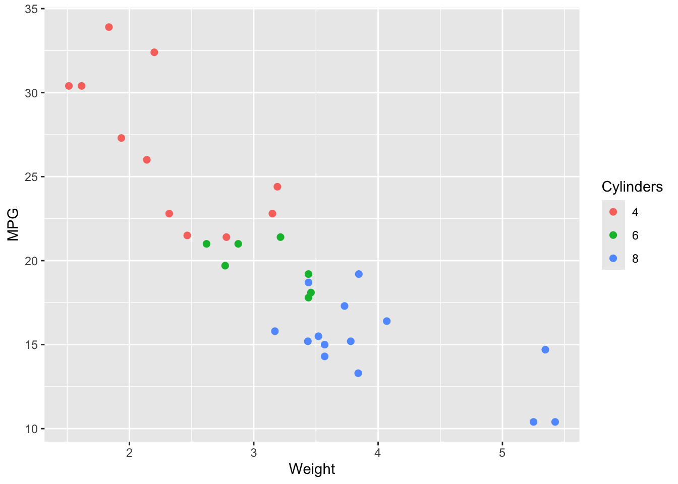
The Export button in the Plots pane can save a figure interactively. Recording ggsave() in the script also preserves the file name and dimensions.
dir.create(here::here("outputs"), showWarnings = FALSE)

ggplot2::ggsave(
  filename = here::here("outputs", "mtcars-scatterplot.png"),
  plot = mpg_plot,
  width = 6,
  height = 4
)
Workflow source: Posit RStudio User Guide: Get Started.
here::here() for reliable paths.getwd()[1] "/Users/jihong/Documents/Projects/website-jihong/teaching/2024-07-21-applied-multivariate-statistics-esrm64503/Lecture01"here::here()[1] "/Users/jihong/Documents/Projects/website-jihong"Use File → New Project to start in a new directory, organize an existing directory, or obtain a project from version control.
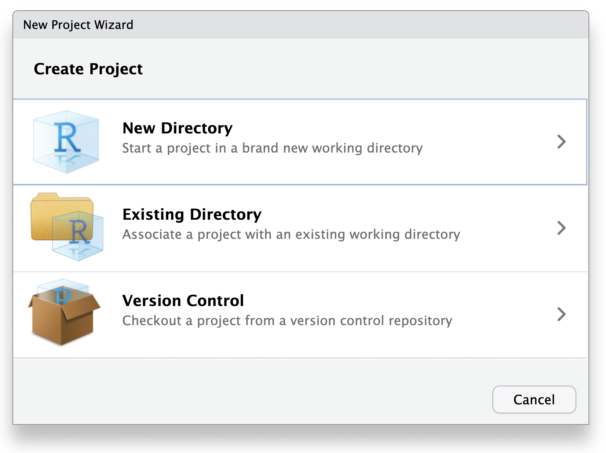
Screenshot source: Posit RStudio User Guide: RStudio Projects.
sessionInfo()R version 4.5.2 (2025-10-31)
Platform: aarch64-apple-darwin20
Running under: macOS Tahoe 26.5.2
Matrix products: default
BLAS: /System/Library/Frameworks/Accelerate.framework/Versions/A/Frameworks/vecLib.framework/Versions/A/libBLAS.dylib
LAPACK: /Library/Frameworks/R.framework/Versions/4.5-arm64/Resources/lib/libRlapack.dylib; LAPACK version 3.12.1
locale:
[1] C.UTF-8/C.UTF-8/C.UTF-8/C/C.UTF-8/C.UTF-8
time zone: America/Chicago
tzcode source: internal
attached base packages:
[1] stats graphics grDevices utils datasets methods base
other attached packages:
[1] here_1.0.2 lubridate_1.9.5 forcats_1.0.1 stringr_1.6.0
[5] dplyr_1.2.0 purrr_1.2.1 readr_2.2.0 tidyr_1.3.2
[9] tibble_3.3.1 ggplot2_4.0.2 tidyverse_2.0.0
loaded via a namespace (and not attached):
[1] Matrix_1.7-4 gtable_0.3.6 jsonlite_2.0.0 compiler_4.5.2
[5] tidyselect_1.2.1 Rcpp_1.1.1 unigd_0.2.0 systemfonts_1.3.1
[9] scales_1.4.0 png_0.1-8 yaml_2.3.12 fastmap_1.2.0
[13] reticulate_1.45.0 lattice_0.22-9 R6_2.6.1 labeling_0.4.3
[17] generics_0.1.4 knitr_1.51 htmlwidgets_1.6.4 rprojroot_2.1.1
[21] tzdb_0.5.0 pillar_1.11.1 RColorBrewer_1.1-3 rlang_1.1.7
[25] stringi_1.8.7 xfun_0.56 S7_0.2.1 otel_0.2.0
[29] timechange_0.4.0 cli_3.6.5 withr_3.0.2 magrittr_2.0.4
[33] digest_0.6.39 grid_4.5.2 hms_1.1.4 lifecycle_1.0.5
[37] vctrs_0.7.1 evaluate_1.0.5 glue_1.8.0 farver_2.1.2
[41] httpgd_2.0.4 rmarkdown_2.30 tools_4.5.2 pkgconfig_2.0.3
[45] htmltools_0.5.9 Use ?function_name or help("function_name") to open documentation in the Help pane. Use example() to run a function’s documented examples.
?mean
help("mean")
example(mean)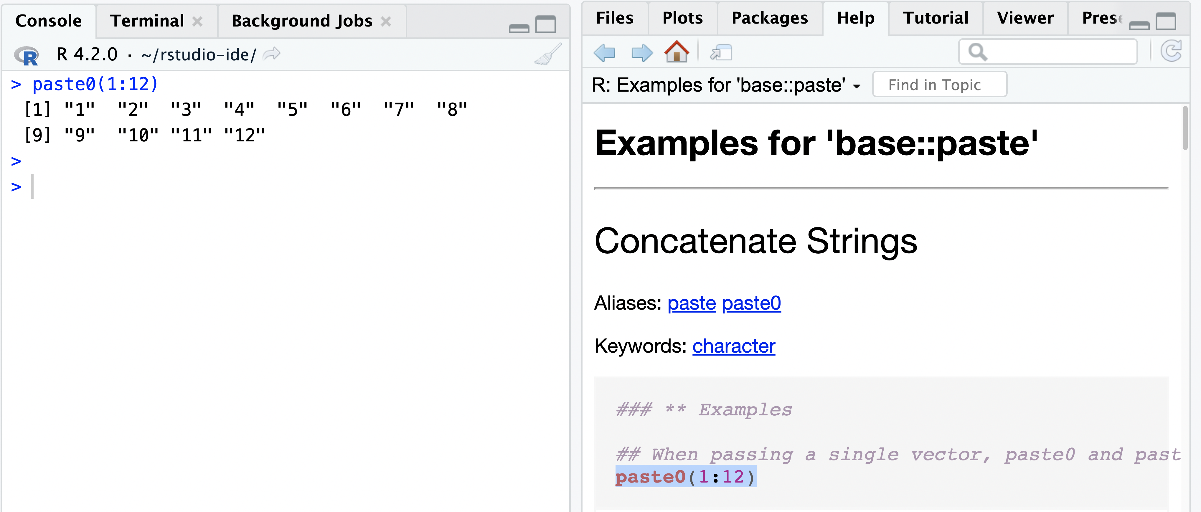
Screenshot source: Posit RStudio User Guide: Pane Layout and Help.
tidyverse (readr, dplyr, tidyr, ggplot2).R scripts so you can rerun and inspect them